Meera Hahn

Creation of tiny images

In this part of the project I implemented one of the simplest image representation forms. I simply read in the image and then resized it to 16 by 16. This then acts as feature representation of the image to feed into the classifier.

Implementation of Nearest Neighbor algorithm

In this part of the project I implemented the Nearest Neighbor algorithm. For this classifier I simply calculated the distance of each test vector to each training vector. Then I select the training vector that was closest to the test vector and predicted the label of the corresponding test image the label of the corresponding training image.
I got the following results using the Nearest Neighbor classifier

1. Tiny Images: Accuracy (mean of diagonal of confusion matrix) is 0.201

Creation of a visual vocabulary

To create the visual vocabulary, I took the training set of images and clustered the it into some given number K clusters. The number K determined how big the visual vocabulary would be and how many groups the SIFT features would be partitioned into. For each image I extracted the SIFT features and added them to a matrix. Then I ran the matrix of all SIFT features through a k-means clustering algorithm with K being the vocab size. Then I save the centroids of the clusters as the visual words for my system. In the visual vocabulary I extraced the SIFT features with a step size of 10 and a size of 8.

Extraction of sift features and creation of a bag of features

To create my bag of features I extracted the SIFT features from each image and then took then found the distance between each feature and each visual word in the vocabulary. I took the visual word that was the closest to the feature and added a count in a histogram to account for the number of times that a visual word was seen in an image. Then I normalized the histogram, which was 1 by vocab size. I returned a matrix of each histogram for each training image. In the creation of a bag of features, I extraced the SIFT features with a step size of 5 and a size of 8.

Implementation of Support Vector Machine classification

Then I implemented the part of the project that trained a linear SVM for each scene category. Since SVM is binary (1 vs all) I needed to build 15 SVMs since there was 15 categories. Then I used the trained SVMs to predicted the scene category of each of the training images and returned the predicted labels. To build and train the SVMs I set all the labels to -1 except for the category I was building the classifier for, which I set to 1. Then for classification of the training images, I ran the features for that image through each of the 15 SVMs and then gave it the label of the SVM which outputted the highest confidence. The SVM classifier takes in the parameter lambda and I set the lamda to 0.00001.
I got the following results using the SVM classifier

1. Bag of SIFT - (vocab of 200): Accuracy (mean of diagonal of confusion matrix) is 0.675

Extra Credit: Testing effects of different vocab sizes

Since the size of the vocabulary was a free parameter I experimented with different sizes. I tried the sizes 10, 50, 100, 500, 1000. The larger the vocab, the longer it takes to build the vocab because it takes longer for k-means to converge, when I built the vocab I build it with step size 50. I also found that to an extent a larger vocab produces higher accuracy. I ran this with the SIFT bag of words features using step size of 10 and the SVM classifier.

1. 10: 0.366
2. 50: 0.548
3. 100: 0.598
4. 200: 0.619
5. 500: 0.629
6. 1000: 0.624

Extra Credit: Implemenation of Cross Validation

For my implementation of cross validation, I combined the training and testing sets into one set. Then I randomly select a set of X number of training images and Y number of testing images. I trained on this using the vocabulary (100 sized) from the original training set and saved the accuracy. I ran this for 10 iterations and then found the average accuracy and standard deviation from the set accuracies of each iteration. The project suggested doing a 100 training samples and 100 testing samples split but I found this much decreased the accuracy from not doing cross validation. I found that increasing the number of training samples, while still randomly choosing them, boosted accuracy. Below I report the accuracy for the split number_of_training/number_of_testing. I ran this using bag of SIFT features and SVM classifier.

1. 100/100: Final accuracy is 0.434, Standard deviation is 0.061
2. 400/200: Final accuracy is 0.581, Standard deviation is 0.046

Spatial Pyramid Feature Representation

Instead of using the bag of SIFT features described above I used a added spatial information to my features. I first calculated the visual vocabulary for the whole photo. Then I calculated the visual vocabulary for each quadrant of the photo. Then I concatinated the visual vocabularys for each of these together. Thus the size of my spatial pyramid of features for each photo was 5 * vocab_size. I found slight improvement over using the normal bag of SIFT features. My result using the spatial pyramid feature representation is as follows:

1. Accuracy (mean of diagonal of confusion matrix) is 0.672

Fisher Vector

Instead of using the bag of SIFT features and the visual vocabulary described above I used a fisher feature encoding scheme. I useed GMM to construct a visual word dictionary based on SIFT features of the training set. Then I used the vl_fisher method to create an encoding of features for each image in the training and testing set. I found vast improvement over all other methods using the fisher vector. My result using the fisher vector is as follows:

1. Accuracy (mean of diagonal of confusion matrix) is 0.755

Results

Results visualization for poorly performing recognition pipeline.

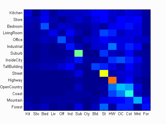
Accuracy (mean of diagonal of confusion matrix) is 0.261

Category name	Accuracy	Sample training images		Sample true positives		False positives with true label		False negatives with wrong predicted label
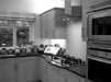
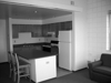
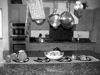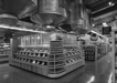
Kitchen	0.080					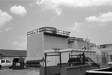Industrial	Forest	Highway	Forest
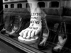
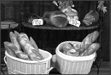
Store	0.040		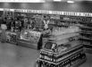			Office	TallBuilding	TallBuilding	Coast
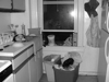
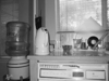
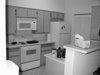
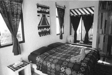
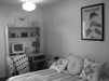
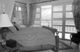
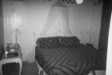
Bedroom	0.200					InsideCity	Store	OpenCountry	Mountain
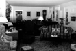
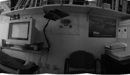
LivingRoom	0.100		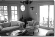			Office	Kitchen	Bedroom	Office
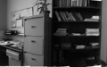
Office	0.190					Mountain	Bedroom	Industrial	InsideCity
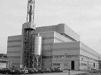
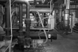
Industrial	0.130					LivingRoom	TallBuilding	InsideCity	Store
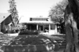
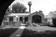
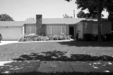
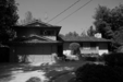
Suburb	0.470					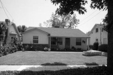Coast	InsideCity	Kitchen	Street
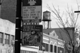
InsideCity	0.030					Suburb	Coast	TallBuilding	Store
TallBuilding	0.180					Store	Forest	LivingRoom	Coast
Street	0.600					Kitchen	Store	Highway	Suburb
Highway	0.750					Suburb	Industrial	Coast	Mountain
OpenCountry	0.310					Forest	Kitchen	Suburb	Coast
Coast	0.400					Mountain	Mountain	InsideCity	OpenCountry
Mountain	0.290					Store	Bedroom	Kitchen	Forest
Forest	0.140					Mountain	Street	Suburb	Kitchen
Category name	Accuracy	Sample training images		Sample true positives		False positives with true label		False negatives with wrong predicted label