Michael Lane

Project 4 / Scene Recognition with Bag of Words

My implementation of this homework differed from the instructions only in that I implemented k-nearest neighbors, rather than simply nearest-neighbor. However, this extra effort clearly does not pay off, as the following table illustrates. Here we have bag-of-sift features with several values for k:

k	1	2	3	4	5
mean accuracy	0.497	0.476	0.443	0.419	0.390

I suggest that this decrease in performance is due to the interface between classes being highly discontinuous.

Here's a full report for k-nearest-neighbors with the best value for k, k=1, with bag-of-sift features.

Confusion Matrix

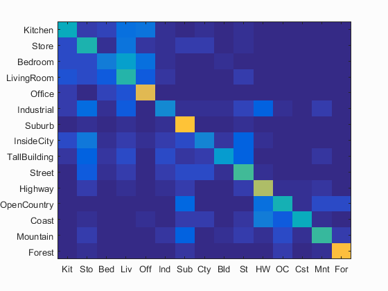
Accuracy (mean of diagonal of confusion matrix) is 0.497

Category name	Accuracy	Sample training images		Sample true positives		False positives with true label		False negatives with wrong predicted label
Kitchen	0.420		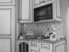			Industrial	Office	Office	Office
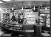
Store	0.460					TallBuilding	Industrial	Kitchen	LivingRoom
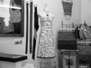
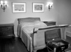
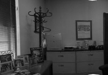
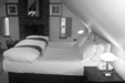
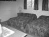
Bedroom	0.220		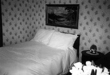		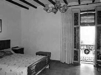	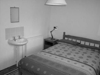LivingRoom	Store	LivingRoom	Office
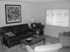
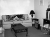
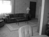
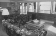
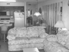
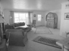
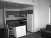
LivingRoom	0.480		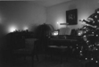			Highway	Street	Street	Bedroom
Office	0.770					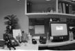Bedroom	Kitchen	Bedroom	Bedroom
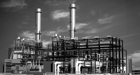
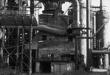
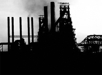
Industrial	0.270					TallBuilding	Street	Street	TallBuilding
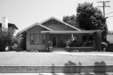
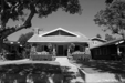
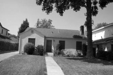
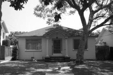
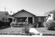
Suburb	0.850		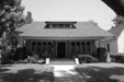			Mountain	Bedroom	Industrial	Coast
InsideCity	0.260					Street	Store	Kitchen	Store
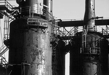
TallBuilding	0.330					Industrial	Bedroom	Industrial	LivingRoom
Street	0.530					Highway	Highway	Store	TallBuilding
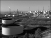
Highway	0.680					Coast	Industrial	Coast	Mountain
OpenCountry	0.440					Mountain	Coast	Mountain	Suburb
Coast	0.410					Highway	Highway	Suburb	OpenCountry
Mountain	0.500					Industrial	Highway	Suburb	TallBuilding
Forest	0.840					Mountain	Mountain	Store	OpenCountry
Category name	Accuracy	Sample training images		Sample true positives		False positives with true label		False negatives with wrong predicted label

As you can see, nearest-neighbor with bag-of-sift performs fairly well for images that are fairly "canonical", such as the forest images. They are canonical in that most forests are the same: many trees, many leaves. Forests tend to contain many high frequency features (leaves, branches) that SIFT encodes well, and thus can be recognized with a high degree of certainty fairly easily. It performs well on "highway" as well, for the same reasons.

Some inexplicably high performance, however, comes from the Suburb images. Most suburban houses do not look the same, from the standpoint of the algorithm. So its (record) high performance goes without explanation.

Running 1-nearest-neighbor on tiny images gave a mean accuracy of about 13%. I will not say more because this particular algorithm because it is not interesting.

Here's the mean accuracy of 1-vs-all SVM linear classifiers using bag-of-sift features, varying the value of lambda.

lambda	10	0.1	0.001	0.0001	0.00001	0.000001
mean accuracy	0.345	0.172	0.419	0.545	0.635	0.649

The accuracy tapers off after 1e-6. This optimum probably has to do with the scale of the feature data, and probably works for all feature data on the same scale.