Project 4: Scene recongition with bag of words

Author: Mitchell Manguno (mmanguno3)

Table of Contents

1. Table of Contents
2. Synopsis
3. Pt. 1: Feature extraction
1. Tiny images
2. Bag of SIFTs
4. Pt. 2: Classifying
1. K-Nearest Neighbors
2. Support Vector Machine
5. Results
   1. Tiny image and KNN
   2. Bag of SIFTS and KNN (best)
   3. Bag of SIFTS and KNN (fast)
   4. Bag of SIFTS and SVM (best)
   5. Bag of SIFTS and SVM (fast)

Synopsis

For this project, 4 seperate image-matching pipelines were implemented with varying degrees of accuracy. Two types of feature extraction methods were utilized: "tiny images", in which the feature vector was the raw pixels of a sized-down image, and "bag of SIFTS", in which a vocabulary of 'words' was generated from a training set, and SIFT features extracted from an image was matched to those 'words'.

Two types of image classification pipelines were utilized in concert with the extraction methods: "k-nearest neighbors", in which each feature was compared against all others, and the mode of the top k was taken as the label, and "support vector machines", in which multiple SVMs were trained on 1 label, and the image features were tested for confidence via each SVM, the top result being taken.

We'll begin with the feature extraction methods.

Pt. 1: Feature extraction

We will discuss the two methods mentioned above: tiny-images and bag-of-SIFTS.

Tiny images

The tiny-image sequence is simple: resize the image, and restructure the N x M matrix of pixel intensities into a N · M x 1 vector. Here is the psuedocode:

R := [], the representative features of all images
for i = 1 ... number of images
    resize image i into N x M
    reshape image i into N · M x 1
    normalize the image vector i
    R[i] = normalized image vector i
return R

Here, the only tunable parameter was the size of the shrunken image. As per recommendation of the file / instructions, I kept this at 16. This provided an accuracy that was within reasonable bounds.

Bag of SIFTs

For this, the sequence is broken up into two parts. First, we build a vocabulary from a training set of words (with kmeans). Second, we iterate over our images, taking SIFT features from each. With each SIFT feature, we try to find the nearest word in our vocabulary. We then have an image and it's associated word/words. Here is the psuedocode:

% Build vocabulary
A := [], all SIFT features of all training images
for i = 1 ... number of training images
    A[i] = SIFT features of training image i

V := the centroids of kmeans(A) as the vocabulary

% Generate the 'bag' of SIFTS
R := [], the representative features of all images
for i = 1 ... number of test images
    S := SIFT features of test image i
    compare S against all V, generating a histogram of the most common words
    R[i] = the histogram of image i
return R

There were two tunable parameters here relating to the performance and accuracy of the feature extraction. These are the SIFT feature detector's 'step' and 'size'. Step refers to the distance the sliding-window moves before it extracts a new feature. Size referes to the size of the window patch used to extract a feature. I found that a step of 12 and a size of 4 found the most accurate features in a relatively good time (~ 11 minutes). In order to make this step slightly faster, I altered the step size to be 14. This put me around 9 minutes of processing time.

Now, onto classification.

let V be the features and labels of all training images
for i = 1 ... number of test images
    let A[i] = extracted features of image i
    compare all A[i] against all V, saving the distances
    save off the k features of least distance (most similarity)
    assign image i with the label that appears most frequently in the k best features

let V be the features and labels of all training images
for i = 1 ... number of labels
    train SVM i on all positive instances of label i in V

for j = 1 ... number of test images
    let A[i] = extracted features of image i
    compare all A[i] against all SVMs, saving the confidences
    save off the SVM of highest confidence (most similarity)
    assign image i with the label of that SVM

Results

And now, onto the results of all runs. For clarity's sake, here is a list of all results (note: 'step' and 'size' in build_vocabulary.m were always 5 and 8,respectively):

• Tiny image and KNN: .201 accuracy (k=3, image size=16)
• Bag of SIFTS and KNN (best): .525 accuracy (k=3, step=12, size=4)
• Bag of SIFTS and KNN (fast): .467 accuracy (k=1, step=14, size=4)
• Bag of SIFTS and SVM (best): .625 accuracy (lambda=.000038, step=12, size=4)
• Bag of SIFTS and SVM (fast): .586 accuracy (lambda=.000038, step=14, size=4)

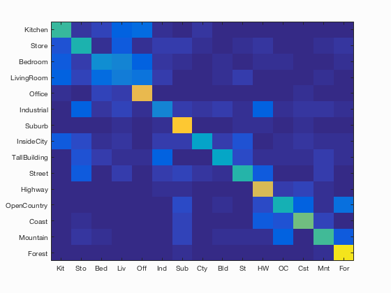
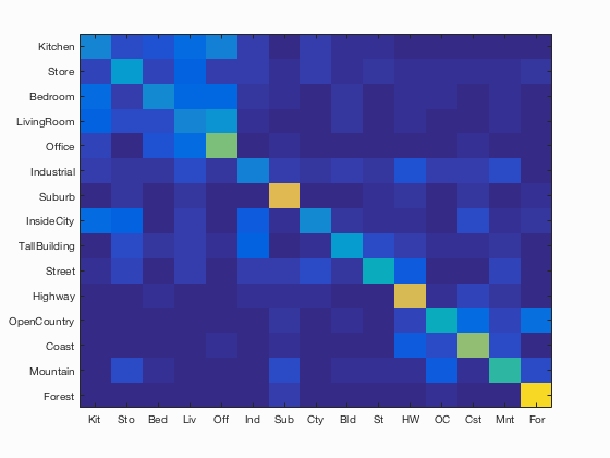
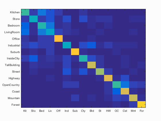
Tiny image and KNN

Scene classification results visualization

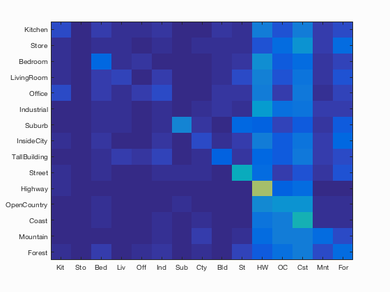
Accuracy (mean of diagonal of confusion matrix) is 0.201

Category name	Accuracy	Sample training images		Sample true positives		False positives with true label		False negatives with wrong predicted label
Kitchen	0.080					Office	Industrial	Coast	Coast
Store	0.010					Forest	Industrial	Highway	Forest
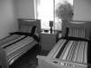
Bedroom	0.150					InsideCity	Kitchen	Highway	OpenCountry
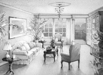
LivingRoom	0.070					Kitchen	Suburb	Coast	Highway
Office	0.060					Bedroom	Street	Coast	Highway
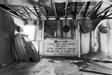
Industrial	0.020					Office	Mountain	Highway	OpenCountry
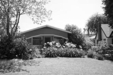
Suburb	0.260					Store	TallBuilding	Forest	Highway
InsideCity	0.080					Coast	Street	Coast	Highway
TallBuilding	0.130					Kitchen	LivingRoom	Highway	LivingRoom
Street	0.420					Forest	Bedroom	InsideCity	Bedroom
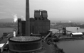
Highway	0.660					TallBuilding	Street	Coast	Kitchen
OpenCountry	0.300					Highway	TallBuilding	Coast	Highway
Coast	0.440					OpenCountry	Store	Bedroom	Mountain
Mountain	0.170					Industrial	TallBuilding	Industrial	Kitchen
Forest	0.170					Mountain	Store	OpenCountry	OpenCountry
Category name	Accuracy	Sample training images		Sample true positives		False positives with true label		False negatives with wrong predicted label

Bag of SIFTS and KNN (best)

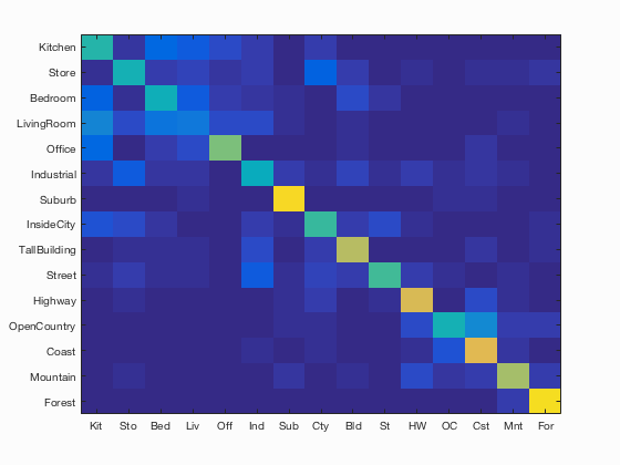
Scene classification results visualization

Accuracy (mean of diagonal of confusion matrix) is 0.525

Category name	Accuracy	Sample training images		Sample true positives		False positives with true label		False negatives with wrong predicted label
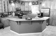
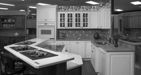
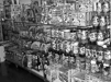
Kitchen	0.510					LivingRoom	Bedroom	Office	Office
Store	0.460					Street	Kitchen	LivingRoom	Street
Bedroom	0.290					LivingRoom	LivingRoom	Industrial	LivingRoom
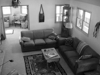
LivingRoom	0.220					Office	Bedroom	Kitchen	Kitchen
Office	0.790					Kitchen	Industrial	LivingRoom	Bedroom
Industrial	0.260					Office	Street	TallBuilding	InsideCity
Suburb	0.860					Industrial	Industrial	LivingRoom	Store
InsideCity	0.360					Industrial	Industrial	Store	LivingRoom
TallBuilding	0.390					Store	OpenCountry	Industrial	Mountain
Street	0.480					InsideCity	LivingRoom	Store	Store
Highway	0.760					Industrial	Bedroom	Office	Industrial
OpenCountry	0.440					Mountain	Mountain	Forest	Forest
Coast	0.580					Industrial	OpenCountry	Highway	OpenCountry
Mountain	0.520					Street	TallBuilding	Highway	Bedroom
Forest	0.950					OpenCountry	OpenCountry	Mountain	Mountain
Category name	Accuracy	Sample training images		Sample true positives		False positives with true label		False negatives with wrong predicted label

Bag of SIFTS and KNN (fast)

Scene classification results visualization

Accuracy (mean of diagonal of confusion matrix) is 0.467

Category name	Accuracy	Sample training images		Sample true positives		False positives with true label		False negatives with wrong predicted label
Kitchen	0.260		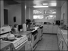			LivingRoom	InsideCity	Office	LivingRoom
Store	0.340					InsideCity	LivingRoom	Kitchen	Office
Bedroom	0.280					Office	LivingRoom	Kitchen	Industrial
LivingRoom	0.260					Suburb	Store	Office	Bedroom
Office	0.600					Industrial	Bedroom	Bedroom	LivingRoom
Industrial	0.240					Store	TallBuilding	TallBuilding	Suburb
Suburb	0.770					OpenCountry	Industrial	Coast	Forest
InsideCity	0.280					TallBuilding	Kitchen	OpenCountry	Suburb
TallBuilding	0.340					Bedroom	Store	Coast	Street
Street	0.410					TallBuilding	TallBuilding	Highway	InsideCity
Highway	0.760					OpenCountry	Street	Coast	LivingRoom
OpenCountry	0.420					Industrial	Coast	Coast	Highway
Coast	0.640					Bedroom	Store	Office	Store
Mountain	0.490					Store	Bedroom	Suburb	Suburb
Forest	0.910					InsideCity	InsideCity	OpenCountry	Store
Category name	Accuracy	Sample training images		Sample true positives		False positives with true label		False negatives with wrong predicted label

Bag of SIFTS and SVM (best)

Scene classification results visualization

Accuracy (mean of diagonal of confusion matrix) is 0.625

Category name	Accuracy	Sample training images		Sample true positives		False positives with true label		False negatives with wrong predicted label
Kitchen	0.510					Office	Industrial	Bedroom	LivingRoom
Store	0.420					TallBuilding	Industrial	InsideCity	Industrial
Bedroom	0.480					Kitchen	LivingRoom	Kitchen	LivingRoom
LivingRoom	0.370					InsideCity	Suburb	Street	Kitchen
Office	0.830					Kitchen	Bedroom	Bedroom	Kitchen
Industrial	0.400					TallBuilding	LivingRoom	Store	Bedroom
Suburb	0.870		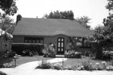			InsideCity	InsideCity	InsideCity	LivingRoom
InsideCity	0.480					Street	Store	LivingRoom	Bedroom
TallBuilding	0.720					Street	InsideCity	Forest	Bedroom
Street	0.650					Store	Bedroom	Industrial	InsideCity
Highway	0.770					Coast	Store	LivingRoom	LivingRoom
OpenCountry	0.510					Coast	Suburb	Forest	Forest
Coast	0.750					Mountain	Bedroom	OpenCountry	Industrial
Mountain	0.720					Industrial	OpenCountry	Forest	Highway
Forest	0.900					Store	TallBuilding	Mountain	Mountain
Category name	Accuracy	Sample training images		Sample true positives		False positives with true label		False negatives with wrong predicted label

Bag of SIFTS and SVM (fast)

Scene classification results visualization

Accuracy (mean of diagonal of confusion matrix) is 0.586

Category name	Accuracy	Sample training images		Sample true positives		False positives with true label		False negatives with wrong predicted label
Kitchen	0.470					LivingRoom	Office	LivingRoom	InsideCity
Store	0.450					InsideCity	Industrial	LivingRoom	Bedroom
Bedroom	0.430					Kitchen	LivingRoom	Kitchen	Coast
LivingRoom	0.210					Kitchen	Store	Store	Store
Office	0.600					Store	Kitchen	LivingRoom	Kitchen
Industrial	0.420					Street	Forest	Store	TallBuilding
Suburb	0.910					Industrial	LivingRoom	LivingRoom	LivingRoom
InsideCity	0.500					Highway	TallBuilding	Store	Store
TallBuilding	0.690					InsideCity	Industrial	Industrial	LivingRoom
Street	0.530					Bedroom	Highway	Store	Highway
Highway	0.760					Street	OpenCountry	Store	InsideCity
OpenCountry	0.450					Street	Coast	Industrial	Mountain
Coast	0.770					OpenCountry	OpenCountry	OpenCountry	Mountain
Mountain	0.670					OpenCountry	LivingRoom	Suburb	TallBuilding
Forest	0.930					Mountain	Mountain	Mountain	Street
Category name	Accuracy	Sample training images		Sample true positives		False positives with true label		False negatives with wrong predicted label