Madeleyne Vaca

Features

Tiny Images

Much like the name suggests, this method involves obtaining a much smaller image representation, say 16X16 pixels, from each of the test images. There are two ways to approach this. You can either take a small chunk of the image as your representation or you can scale the image down to a small size. As I believed that there were components of the image that even at a scaled down version would still be important, I opted to scale the images rather than take just a chunk. To make it easier to store multiple images in the same matrix, I converted this 16X16 matrix to a 1X256 matrix.

Bag of Sift

This method involves extracting sift features from the images with vl_dsift, calculating and assigning the sift features to their nearest vocab feature, and constructing a histogram of frequency of vocab use. The vocabulary is a clustering of sift features that were extracted from the training images. There are quite a few paramters that can be tweaked in this step to achieve different accuracies, namely step size and bin size whilst extracting the sift features and the size of the vocabulary. I began with a vocab size of 250, a step size of 22, and a bin size of 4 to prove that my code could work and reduced my steps in increments of 4 until the accuracy of my outputs and the time for my code to run were both within the requirements. Below is the code for how I extract the features and create the histograms for each feature.

    [locations, SIFT_features] = vl_dsift(single(img), 'step', 8, 'size', 4, 'fast');
    distances = vl_alldist2(double(SIFT_features), double(vocab));
    [val indices] = min(distances, [], 2);
    indices = indices';
    dim = size(indices);
    histogram = zeros(1, vocab_size);
    for j = 1:dim(2)
       histogram(indices(j)) = histogram(indices(j)) + 1; 
    end
    histogram = norm(histogram);

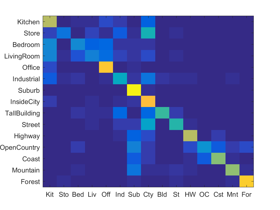
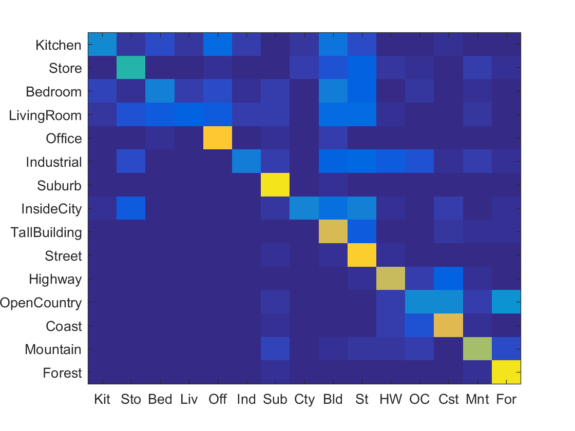
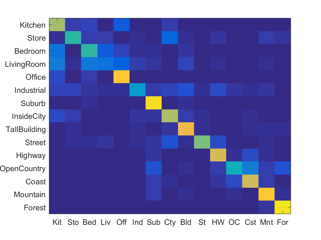
As you can see, I ended up with a step size of 6. Below are some of the confusion tables that my iterative process came up with from worst to best accuracy.

Results in a table

Classifiers

1-Nearest Neighbor

This classifier is rightfully named as all it does is find the training image category that on average has the most similar features to the feature being tested. This is where the tiny image or visual words come in.

SVM classifier

This classifer is structurally a lot more complicated than Nearest Neighbor. First, an SVM has to be trained for each of the 15 categories and the hyperplane parameters, W and B, have to be stored for each one. There is a parameter, called lambda, that can be tweaked here to improve accuracy. I began with .001 and dropped by .0002 until reaching a value of .0005 that I found to give me the best accuracy. Below is the code for training one of these SVMs.

    bin_labels = double(strcmp(categories{i},train_labels));
    bin_labels(bin_labels == 0) = -1;
    [W B] = vl_svmtrain(train_image_feats',bin_labels', lambda);%[W B]
    W_matrices(i,:)= W; 
    B_vals(i) = B;

After the training, I iterate through all of the test image features and compute the confidences for each category using the hyperplane parameters found by the code above. The category that has the highest confidence value is the one that is predicted for this test feature. Once again, the code for this loop is found below.

    confidences = [];
    for j = 1:num_categories
        conf = dot(W_matrices(j,:)', test_image_feats(feat,:)) + B_vals(j);
        confidences = [confidences conf];
    end
    [vals ind] = max(confidences);
    predicted_categories(feat) = categories(ind);

Results for Different Feature and Classifier Pairs

The parameters for these results are the same as discussed above.

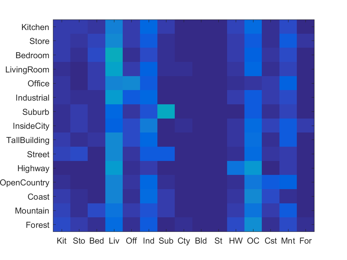
SVM & Tiny Image Accuracy .144

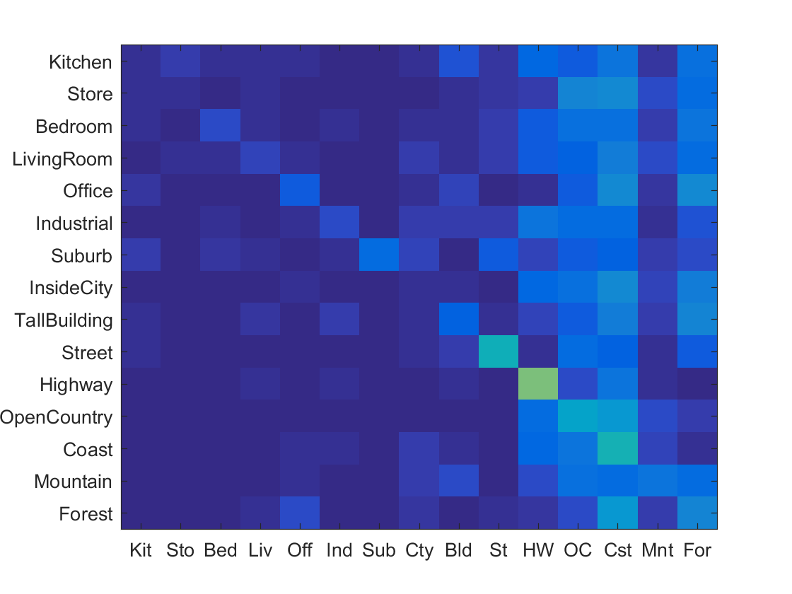
NN & Tiny Image Accuracy .201

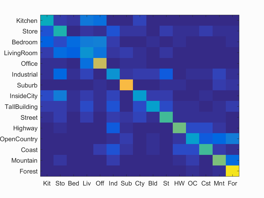
SVM & Bag of Sift Accuracy .652

NN & Bag of Sift Accuracy .501

Results visualization for decently performing recognition pipeline (NN & Bag of Sift).

Accuracy (mean of diagonal of confusion matrix) is 0.501

Category name	Accuracy	Sample training images		Sample true positives		False positives with true label		False negatives with wrong predicted label
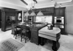
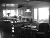
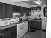
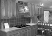
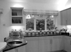
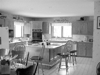
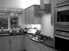
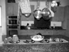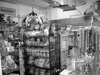
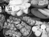
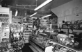
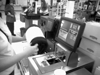
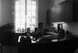
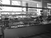
Kitchen	0.410					InsideCity	TallBuilding	Store	Office
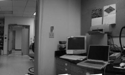
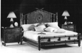
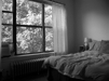
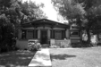
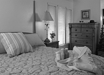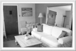
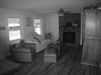
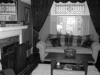
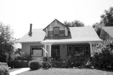
Store	0.460					Bedroom	LivingRoom	Kitchen	Suburb
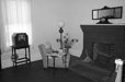
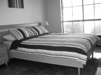
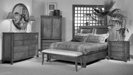
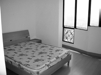
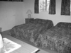
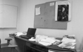
Bedroom	0.160		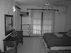			Kitchen	OpenCountry	Industrial	LivingRoom
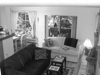
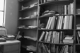
LivingRoom	0.300		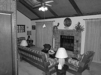			Bedroom	Office	Bedroom	Store
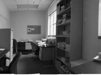
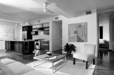
Office	0.720		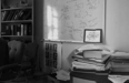			LivingRoom	Kitchen	InsideCity	Kitchen
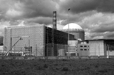
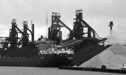
Industrial	0.310		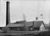			Store	TallBuilding	Store	Kitchen
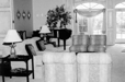
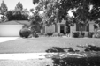
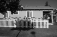
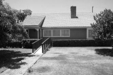
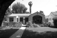
Suburb	0.820		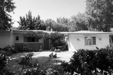			Office	LivingRoom	Office	Mountain
InsideCity	0.340					TallBuilding	TallBuilding	Coast	TallBuilding
TallBuilding	0.350					Industrial	Kitchen	Store	Bedroom
Street	0.520					Store	TallBuilding	Coast	Store
Highway	0.580					OpenCountry	Bedroom	Industrial	Coast
OpenCountry	0.350					Mountain	Highway	Mountain	Forest
Coast	0.530					Industrial	Highway	Suburb	Office
Mountain	0.600					Suburb	OpenCountry	Industrial	Forest
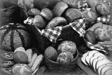
Forest	0.940					Store	Mountain	OpenCountry	Mountain
Category name	Accuracy	Sample training images		Sample true positives		False positives with true label		False negatives with wrong predicted label