Project 4 / Scene Recognition with Bag of Words

Tiny images + Nearest neighbor classifier

Tiny image is a simple image representation. I just resized the given image into 16 x 16 resolution. Nearest neighbor classifier is also easy to implement. We just find all pairs distances between test images and training images and classify each test image to the category of its nearest neighbor. Since tiny image is not a good represeantation, I only got about 0.191 accuracy.

Bag of SIFT + Nearest neighbor classifier

The first step for bag of SIFT representation is to build a vocabulary of visual words. I used all the training images provided to build a representative set of SIFT features (using a high step size of 50). Next, I clustered these into 200 clusters using kmeans. These 200 centroids represent our vocabulary and are saved to disk to avoid recomputation each time.
The second step is to represent training and test images as histograms of visual words. We densely sample SIFT features (lower step size of 10) from each of them. Each SIFT feature votes for the visual word that it is closest to and this way we build our histogram. We normalize the final histogram and this becomes our image representation for classification. Using nearest neighbor classification and this representation, I got about 0.483 accuracy. Removing 'fast' from vl_fucntions, increasing vocabulary size to 400, reducing step sizes to 30 and 6 got me over 50% accuracy but this takes more time.

Bag of SIFT + 1-vs-all SVM classifier

This time we again use bag of sift features but use SVMs for classification. We train one SVM for each category against all others we have in the given clasification problem. I used vl_svmtrain to get the SVM classifiers with LAMBDA value of 0.00001. Once we have the 15 SVMs, for each test image we calculate the confidence or distance using each of the classfiers. The test image is classified to category which gives the highest confidence. I got a huge boost to my accuracy but this takes more time. using SVMs, I got about 0.613 before optimizing my parameters.

Next I optimized the parameters. I increased vocabulary size to 400, used step sizes of 30 (for vocab) and 6 (for histogram). I changed LAMBDA to 0.000001. I still used 'fast' versions of vl algorithms since it was suggested to keep the total computation under 10 minutes. These changes bumped my accuracy to 0.672. This is the best I got without extra credit work.

Extra credit I / Single Level spatial information

I split the given image into four parts and independently built bag of sift features for each of them(eq to level 1 single level described by Lazebnik et al 2006). I stacked these four histograms and used them as my features for classification.
Adding this simple spatial information helped increase accuracy over my normal bag of sift features.However, I observed good bumps in accuracy when I was using sub-optimal parameters. My accuracy increased from 0.613 with sub-optimal bag of sifts to 0.66. However, with optimal parameters my accuracy just increased from 0.672 to 0.69.

Extra credit II / Soft Assignment

Instead of each SIFT feature voting for just one visual word in the histogram construction, soft assignment allows distance-weighted vote to multiple bins (say r bins). I chose r = 3 meaning each SIFT feature votes for 3 closest visual words. I used exp(-d*d/sigma) weighting function for the votes, where d is distance and I chose sigma = 5 x 10^(9).
This addition also boosted my accuracy a bit. However like in previous case, the bump was 1%-2% when I am already using optimal parameters for bag of sifts. Using spatial information, soft assignment and removing the 'fast' variable in vl_functions, I got an accuracy of 0.723.

Extra Credit III / Fisher Encoding

Fisher vector is an alternative representation which is more sohisticated than the popular bag of sifts. First, we build a GMM model using samples of SIFT features from images in our database. I set number of clusters to 400. This step is equivalent to vocabulary building in bag of sifts model. Next, we use parameters obtained from this step to build fisher encoding for a given image. The dimensions of this encoding for each image would be 128*400*2.
I got excellent results using fisher encoding and same parameters for others as before. My accuracy was 0.749 which is the best I could get in the project and I display the results below.

Scene classification results visualization

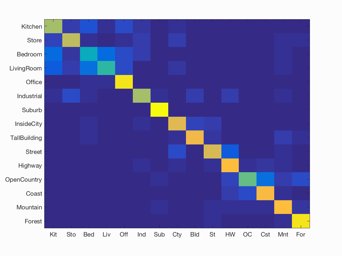
Accuracy (mean of diagonal of confusion matrix) is 0.749

Category name	Accuracy	Sample training images		Sample true positives		False positives with true label		False negatives with wrong predicted label
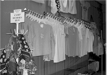
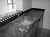
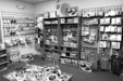
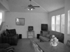
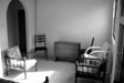
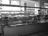
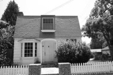
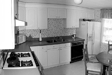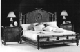
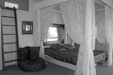
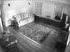
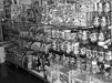
Kitchen	0.660					Bedroom	Store	Bedroom	Bedroom
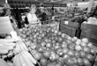
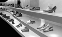
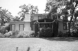
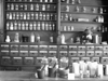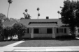
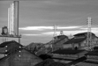
Store	0.710					TallBuilding	Bedroom	Industrial	Street
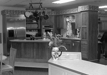
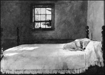
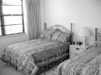
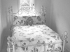
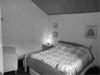
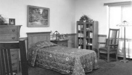
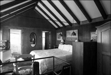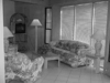
Bedroom	0.420					Highway	LivingRoom	LivingRoom	Kitchen
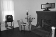
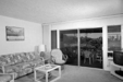
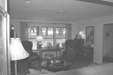
LivingRoom	0.490		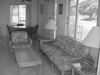			Bedroom	Bedroom	Office	Kitchen
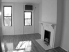
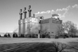
Office	0.950					Bedroom	LivingRoom	LivingRoom	Bedroom
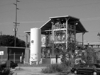
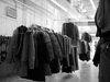
Industrial	0.670		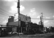			Store	Highway	Suburb	TallBuilding
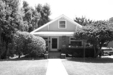
Suburb	0.990		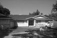			Street	Bedroom	TallBuilding
InsideCity	0.780					Kitchen	Street	TallBuilding	Industrial
TallBuilding	0.800					Kitchen	Store	Mountain	InsideCity
Street	0.760					Highway	TallBuilding	InsideCity	Mountain
Highway	0.830					Street	Street	Forest	Suburb
OpenCountry	0.570					Mountain	Industrial	Mountain	Coast
Coast	0.820					Mountain	OpenCountry	Mountain	Highway
Mountain	0.830					LivingRoom	Coast	Street	Coast
Forest	0.950					TallBuilding	Store	Street	Street
Category name	Accuracy	Sample training images		Sample true positives		False positives with true label		False negatives with wrong predicted label