Bag of SIFT representation and linear SVM classifier:

For Bag of SIFT representation, the vocabulary needs to be created from the training images. The sift features from each training image are extracted with a step size of 16. The large step size is chosen to save computation time. Best accuracy is obtained with vocabulary size of 100. The accuracy vs vocabulary size chart is discussed in bells and whistles. So in conclusion, vocabulary size of 100 and step size of 16, gives the best accuracy while taking modest time to build the vocabulary.

Next we take all training images and densely sample sift features from each image. For a given image, each of these features will be binned into clusters of the vocabulary to which it is closest to. The histogram is then normalized. Thus we get a set of train image features. Repeat this for the test images and get the test image features. The step size used in extracting the sift features here, is 8, as we need a dense sampling for better accuracy. The code used for this step is get_bags_of_sifts.m.

Now, using the train image features and train image labels, we need to find the labels for the test image features. For this classification, linear SVM is used here. Regularization parameter LAMBDA is chosen to be 0.00001. Finally, we get an accuracy of 0.6052. However, when step size of sift used to obtain train image features and test image features in get_bags_of_sifts.m is changed to 4 and when LAMBDA is set to 0.0000008, while keeping the vocabulary of size 100 built using step size of 16, we get an accuracy of 0.6524.

Bells and Whistles: Checking performance with different vocabulary sizes:

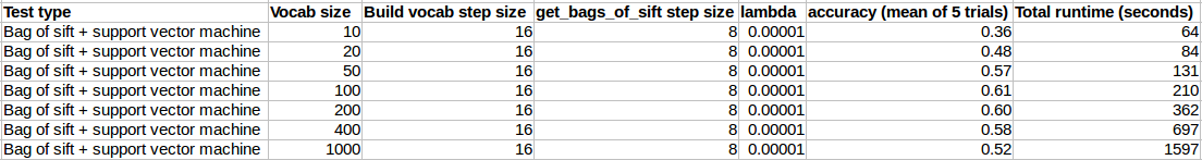
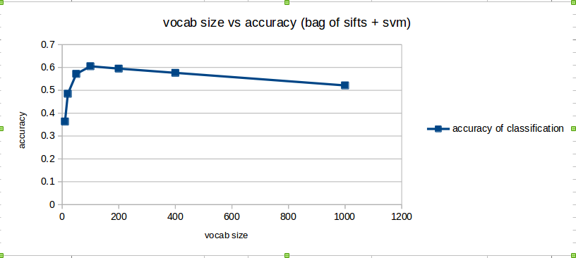
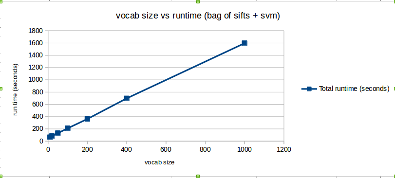
In order to check the effect of varying the vocabulary size on the accuracy and total run time, we fix all the parameters of the system except vocabulary size. Here we use Bag of SIFT representation and linear SVM classifier. We fix step size of sift feature extraction at 16 during building the vocabulary. We fix the step size of sift feature extraction at 8 during creation of train image features and test image features using get_bags_of_sifts.m. We fix LAMBDA of SVM at 0.00001. We use vocabulary sizes of 10, 20, 50, 100, 200, 400, 1000 and compute the accuracy obtained and the total time taken (excluding time taken to build vocabulary).The following table and the two scatter plots display the observations obtained.

Bells and Whistles: Use cross-validation to measure performance:

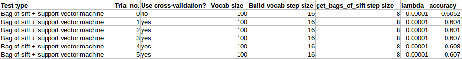
Here cross-validation is used to measure performance rather than the fixed test / train split provided by the starter code. The train and test images for each category are combined and they are shuffled. Now from this shuffled image set per category, 100 images are taken to be the train images for that category and the other 100 are taken to be the test images for that category. This way every time the project is executed, the train images and test images keep changing within each category. In order to check the accuracy of the model with cross-validation, we fix all the parameters of the system. Here we use Bag of SIFT representation and linear SVM classifier. We fix vocabulary size at 100, step size of sift feature extraction at 16 during building the vocabulary. We fix the step size of sift feature extraction at 8 during creation of train image features and test image features using get_bags_of_sifts.m. We fix LAMBDA of SVM at 0.00001. We compute the accuracy obtained. The following table displays the observations obtained. The first entry in the table is obtained using the original fixed train and test images.

Bells and Whistles: Use of sift features at multiple scales:

We use sift features at multiple scales to improve accuracy. We use 6 scales with downsize factor of 0.9. i.e. every image is downsized by 0.9^scale_level and the histogram of the original image along with the histograms of the smaller resolutions of that image are calculated and concatenated to form the new feature vector as bag of sifts. Here we use linear SVM classifier. We fix vocabulary size at 100, step size of sift feature extraction at 16 during building the vocabulary. We initially set the step size of sift feature extraction at 8 during creation of train image features and test image features using get_bags_of_sifts.m. But step size at every scale is reduced by 0.9^scale_level, in order to keep the sift feature sampling dense. We fix LAMBDA of SVM at 0.00001. The accuracy increases from 0.605 to 0.638.

Bells and Whistles: Use of spatial pyramid feature representation:

We use spatial pyramid feature representation in order to improve accuracy. We use 2 levels of pyramid. i.e. every image is divided into 4 equal sub images and the histogram of the original image along with the histograms of the 4 subimages are calculated and concatenated to form the new feature vector as bag of sifts. Here we use linear SVM classifier. We fix vocabulary size at 100, step size of sift feature extraction at 16 during building the vocabulary. We fix the step size of sift feature extraction at 8 during creation of train image features and test image features using get_bags_of_sifts.m. However the step size for the 4 subimages of every image is set to half of the original step size, in order to keep the sift feature sampling dense. We fix LAMBDA of SVM at 0.00001. The accuracy increases from 0.605 to 0.6648.

Bells and Whistles: Use of GIST descriptors along with bag of sifts:

Gist descriptor for each image is obtained and appended or concatenated to the image's histogram of sift feature count obtained from bag of sifts. So the new feature vector for the test and train images consists of a histogram and a gist descriptor, which proves to give more accuracy then just the histogram. Here we use linear SVM classifier. We fix vocabulary size at 100, step size of sift feature extraction at 16 during building the vocabulary. We fix the step size of sift feature extraction at 4 during creation of train image features and test image features using get_bags_of_sifts.m. We fix LAMBDA of SVM at 0.0001. The accuracy increases to 0.7336.

Citations:

Beyond Bags of Features: Spatial Pyramid Matching for Recognizing Natural Scene Categories. Lazebnik et al 2006. http://www.cs.unc.edu/~lazebnik/publications/cvpr06b.pdf

Modeling the Shape of the Scene: A Holistic Representation of the Spatial Envelope. Aude Oliva et al. http://people.csail.mit.edu/torralba/code/spatialenvelope/

Scene classification results visualization

Obtained using bells and whistles: Use of GIST descriptors along with bag of sifts:

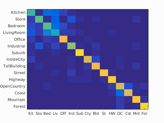
Accuracy (mean of diagonal of confusion matrix) is 0.735

Category name	Accuracy	Sample training images		Sample true positives		False positives with true label		False negatives with wrong predicted label
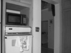
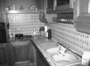
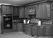
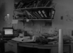
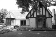
Kitchen	0.510					Industrial	Suburb	InsideCity	Bedroom
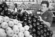
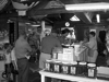
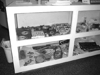
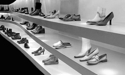
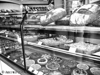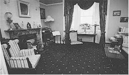
Store	0.560					Industrial	LivingRoom	Suburb	LivingRoom
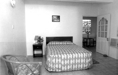
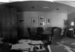
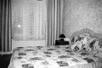
Bedroom	0.550					LivingRoom	LivingRoom	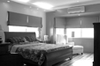Office	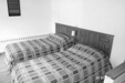Mountain
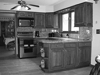
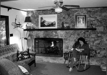
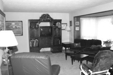
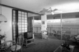
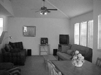
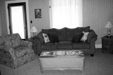
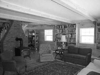
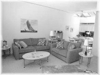
LivingRoom	0.430		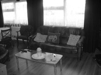			Industrial	Kitchen	Kitchen	Industrial
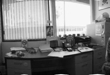
Office	0.820		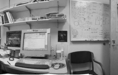			InsideCity	Kitchen	Kitchen	Kitchen
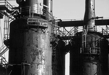
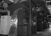
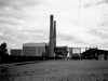
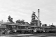
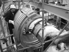
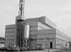
Industrial	0.630					Highway	Bedroom	Store	Kitchen
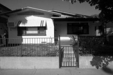
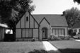
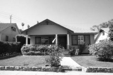
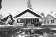
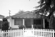
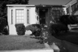
Suburb	0.930		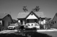			Highway	Store	Kitchen	LivingRoom
InsideCity	0.750					Street	Suburb	Kitchen	TallBuilding
TallBuilding	0.800					InsideCity	InsideCity	Bedroom	Industrial
Street	0.850					InsideCity	LivingRoom	Industrial	LivingRoom
Highway	0.890					LivingRoom	Coast	InsideCity	LivingRoom
OpenCountry	0.760					Forest	Coast	Forest	Forest
Coast	0.780					OpenCountry	OpenCountry	OpenCountry	OpenCountry
Mountain	0.860					Store	Store	OpenCountry	OpenCountry
Forest	0.910					Mountain	Highway	OpenCountry	Mountain
Category name	Accuracy	Sample training images		Sample true positives		False positives with true label		False negatives with wrong predicted label