Project 4 / Scene Recognition with Bag of Words
In this project, we used the bag of visual words model to classify images into one of 15 categories. We started with a simple sample of the image with tiny images which takes a 16x16 patch of an image and uses the nearest neighbor classifier to find the closest test image to assign its class to. Then we moved to implement bag of sifts which creates sift features for every image and used the nearest neighbor classifier once again to find the closest match for each image. Finally we used the svm classifier along with bag of sifts to achieve the best results.
Building Vocabulary
For building a vocabulary, I simply used vl_sift and vl_kmeans to group sift features together. We had a vocabulary size of 200. I started with using a step size of 3 for vl_sift. This took >8 hours to run. So I changed to a step size of 10 for building vocab but found that smaller SIFT features tend to have slightly better result. I had a slightly better accuracy with step size of 3 than with step size of 10. (0.631 vs 0.667). The code included in the project uses a step size of 10 for building the vocabulary because step size of 3 was taking too long.
Tiny Images + Nearest Neighbor
The tiny images + nearest neighbor pipeline was the worst performing pipeline which is unsurprising since it doesn't do anything very intellgent during image sampling. It simply creates a 16x16 patch of the image. This pipeline achieved 0.201 accuracy. The steps followed are listed below:
- Create 16x16 patch of image
- For every patch find the nearest neighbor (euclidean) in the image space.
- Assign that image the class of it's nearest neighbor.
One advantage of 1-nearest neighbor is that it's very simple. It requires no training and can be used to created any boundary. However, the downside is that it's not very flexible.
Bag of Sifts + Nearest Neighbor
For this pipeline, I retrieved SIFT features for each image and tried to match those SIFT features to the training data SIFT features. Then using vl_alldist2 and sort, I found the vocab words that were closest to the SIFT features. Then, I created a histogram for each image of classes that match the sift features for each image.
% SIFT + closest visual word + histogram creation
for i=1:n
   [locations, SIFT_FEATURES] = vl_dsift(single(imread(image_paths{i})), 'step', 8);
   dist = vl_alldist2(single(SIFT_FEATURES), vocab);
   % sift x vocab
   % Row-wise sort bc of vl_alldist2 - Entries in 1st column are closest
   % cluster centers
   [S, I] = sort(dist, 2);
   histogram = zeros(1, k);

   for ind=1:size(I, 1)
       histogram(1, I(ind, 1)) = histogram(1, I(ind, 1)) + 1;
   end
   image_feats(i, :) = histogram/norm(histogram, 2);
end
The code above shows the core of the bag of sifts algorithm starting with retrieving SIFT features for every image then creating a histogram of closest vocab matches for each image. For this pipeline, I chose a step size of 8 which gave me 0.511 accuracy. I found that with a smaller step size such as 4-5, I got a slightly higher accuracy but an overall slower pipline. Step size of 8 for sift features got my pipeline working with acceptable accuracy in 10 minutes.
Bag of Sifts + SVM
For this pipeline, I followed the same procedure as above for retrieving SIFT features to testing and training images. The only difference is the classifier which is SVM in this case. This pipeline provided the highest accuracy. I chose a step size of 8 which gave me .631 accuracy. I found that with a smaller step size such as 4-5, I get higher accuracy but an overall slower pipline. Step size of 8 got my pipeline working with acceptable accuracy in 10 minutes. The lambda that seemed to work best for me around 0.00001. Anything larger than that gave poorer results. Overall, the range 0.00001 - 0.00006 seemed to work very well. The results are highlighted in the confusion matrix and images below. The parameters that produced the best accuracy are a step size of 8 for finding SIFT features in get_bag_of_sifts.com and a lambda of 0.00001 in svm_classify when training the svm model.
Results for Bag of Sifts + SVM

Accuracy (mean of diagonal of confusion matrix) is 0.631
| Category name | Accuracy | Sample training images | Sample true positives | False positives with true label | False negatives with wrong predicted label | ||||
|---|---|---|---|---|---|---|---|---|---|
| Kitchen | 0.490 |  |
 |
 |
 |
 InsideCity |
 Office |
 Bedroom |
 Bedroom |
| Store | 0.360 |  |
 |
 |
 |
 LivingRoom |
 Bedroom |
 Kitchen |
 InsideCity |
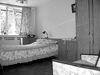
| Bedroom | 0.480 |  |
 |
 |
 |
 Street |
 LivingRoom |
 Kitchen |
 Store |
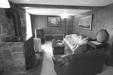
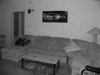
| LivingRoom | 0.360 |  |
 |
 |
 |
 Office |
 Store |
 TallBuilding |
 Street |
| Office | 0.780 |  |
 |
 |
 |
 Kitchen |
 Kitchen |
 Bedroom |
 LivingRoom |
| Industrial | 0.460 |  |
 |
 |
 Suburb |
Store |
 Kitchen |
 Suburb |
|
| Suburb | 0.890 | 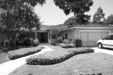 |
 |
 |
 |
Industrial |
 InsideCity |
 Coast |
 Mountain |
| InsideCity | 0.520 |  |
 |
 |
 |
 Store |
 Street |
 Kitchen |
 Store |
| TallBuilding | 0.790 |  |
 |
 |
 |
 InsideCity |
 Street |
 LivingRoom |
 Industrial |
| Street | 0.550 |  |
 |
 |
 |
 LivingRoom |
 Bedroom |
 InsideCity |
 Bedroom |
| Highway | 0.750 |  |
 |
 |
 |
 Mountain |
 Industrial |
 Coast |
 Street |
| OpenCountry | 0.540 |  |
 |
 |
 |
 Coast |
 Coast |
 Bedroom |
 Coast |
| Coast | 0.810 |  |
 |
 |
 |
 OpenCountry |
 OpenCountry |
 Suburb |
 Highway |
| Mountain | 0.780 |  |
 |
 |
 |
 Store |
 OpenCountry |
 Coast |
 TallBuilding |
| Forest | 0.910 |  |
 |
 |
 |
 Store |
 OpenCountry |
 TallBuilding |
 OpenCountry |
| Category name | Accuracy | Sample training images | Sample true positives | False positives with true label | False negatives with wrong predicted label | ||||