Project 4 / Scene Recognition with Bag of Words
In this project the objective was to train a scene classifier and recognize scenes. To do this we implemented the following solutions:
- Tiny image features, we resize the images to a fixed small scale.
- Implemented a 1-nearest neighbor classifier.
- Implemented SIFT vocabulary and bag of words features.
- Implemented a multi-class SVM classifier.
- Fine tuned the bin size parameter for SIFT and the SVM regularization parameter.
- Tested the performance of SIFT bag of words and SVM using multiple vocabulary sizes.
- Implemented spatial pyramid features for SIFT bag of words.
- Implemented Fisher Encoding that replaces bag of words.
- Implemented GIST features and tested them alongside SIFT features with Fisher Encoding.
- Implemented a non-linear SVM with an RBF kernel.
Tiny images and nearest neighbor
I did not do anything fancy for this part and just resized the images using matlab functions. The nearest neighbor classifier is just a 1-nearest neighbor classifier.
SIFT, SVM and fine-tuning
I implemented SIFT vocabulary extraction and SIFT bag of words which essentially is just extracting the SIFT features from the images and building a histogram of counts of the nearest neighbors of these features. I had a problem for a while where I tried to use the histcounts matlab function and my accuracies were not good enough. The problem that we could not even detect with the TAs was that the function had unexpected behavior. It was discretizing the continuous range [1 max_nearest_neighbor_index] into vocab_size bins instead of binning vocab_size integers which means that if the max_nearest_neighbor_index of an image was less than vocab_size features were being binned incorrectly. After debuggin my code I found out this was the problem and just implemented a histogram count on my own which worked.
I then fine-tuned the regularization parameter of SVM before fixing the binning problem. The fine-tuned parameter 0.00001 worked well in next parts.
| lambda | accuracy |
|---|---|
| 1 | 0.395 |
| 0.1 | 0.316 |
| 0.01 | 0.307 |
| 0.001 | 0.427 |
| 0.0001 | 0.535 |
| 0.00005 | 0.569 |
| 0.00001 | 0.572 |
| 0.000001 | 0.559 |
| 0.0000001 | 0.492 |
| 0.00000001 | 0.469 |
I fine-tuned the size of the SIFT bins after fixing the binning issue. I used step 10 for building the vocabulary and step 10 for testing. The fast parameter was also used for both. The SVM classifier was used. The bin size used for the rest of the probject is 8x8.
| bin size | accuracy |
|---|---|
| 3x3 | 0.625 |
| 8x8 | 0.649 |
| 16x16 | 0.639 |
| 32x32 | 0.590 |
| 64x64 | 0.491 |
Different vocabulary sizes
I tested the performance of my pipeline using different vocabulary sizes. I used step of 1 to build the vocabularies which ran overnight and took a long time (I wrote a script to build several vocabs). The size of the bins was 3x3 which is the default for vl_sift. I used this size of bins because I did this before optimizing the bin size. To test I used a step of 10 and the fast parameter.
| vocab_size | accuracy | time to test |
|---|---|---|
| 10 | 0.344 | 38s |
| 20 | 0.471 | 45s |
| 50 | 0.545 | 68s |
| 100 | 0.589 | 107s |
| 200 | 0.615 | 194s |
| 400 | 0.641 | 334s |
| 1000 | 0.639 | 786s |
As we can see the performance climbs until hitting diminishing returns at around the vocab size of 400. The performance then starts to slightly suffer from increasing vocab sizes. The time taken to test is also much higher for higher vocab sizes and the time to build is extremely long for large vocab sizes. A vocab size of 200 is very adequate.
SIFT with spatial pyramids
I implemented SIFT with spatial pyramids. In essence I extract SIFT features from the image, then subdivide the image in four parts and extract the SIFT features of these four parts and count and concatenate the feature vectors and then subdivide it into 16 parts, extract the features and count and concatenate again. Using SVM with lambda 0.00001, vocab size 200, step vocab building 3, 8x8 bins and step 5 for SIFT feature extraction we have the following results.
| accuracy | |
|---|---|
| without pyramids | 0.672 |
| with pyramids | 0.701 |
Fisher encoding
I implemented fisher encoding by creting a get_vl_gmm script and a get_fisher_sifts script. The get_vl_gmm script essentially builds the vocabulary for fisher encoding using the vl_gmm function. The get_fisher_sifts creates the feature vectors using the vl_fisher functions. I tuned the vocabulary size for my fisher encoding.
| vocab_size | accuracy |
|---|---|
| 30 | 0.703 |
| 60 | 0.726 |
| 100 | 0.726 |
| 150 | 0.725 |
Same effect of diminishing returns. So we pick a vocabulary of 60. Note that the pipeline runs much faster and that we are using steps of 10 to extract SIFT features, and still getting good accuracies. I tried step 5 for the SIFT extraction and I got an accuracy of 0.741.
I tried to implement the same idea of using spatial pyramids with Fisher encoding. I implemented the program but the results were not any better or worse. I think Fisher encoding has some sort of spatial information encoding that is redundant with spatial pyramids.
GIST
I added GIST descriptors for images using Oliva and Torralba's code. The good part is that a vocabulary does not need to be built for GIST and we can compare images directly. I used GIST descriptors alongside SIFT features encoded with Fisher vectors. I had a slight accuracy increase.
| accuracy | |
|---|---|
| SIFT w/ Fisher Encoding | 0.741 |
| SIFT w/ Fisher Encoding + GIST | 0.743 |
Non-linear SVM with RBF kernel.
Using Olivier Chapelle's matlab code I implemented a non-linear svm classifier using a gaussian RBF kernel. I compute the kernel using the training data with the kernel function that I found in wikipedia, train the classifier 1 vs all and then find the labels of the test data by first computing the kernel for the test features and computing labels = weights * kernel_test + biases.
My final result is 100% accuracy which had me thinking that I was cheating and using the test labels. I checked my code several times and can't find the moment where the classifier is cheating but I am pretty sure that it is because it gets 100% even with tiny image features. I reviewed the code extensively with a TA but couldn't find where the issue lies. If I change the sigma parameter to 100 I don't get 100% anymore but with a sigma parameter of 1 and lambda = 0.00001 I get 100% accuracy.
I present my most accurate code with SIFT and fisher vector encodings + GIST using a step of 3, bin size 8x8 and the fast parameter which gives me an accuracy of 0.752.
Scene classification results visualization
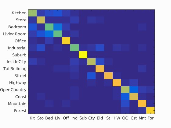
Accuracy (mean of diagonal of confusion matrix) is 0.752
| Category name | Accuracy | Sample training images | Sample true positives | False positives with true label | False negatives with wrong predicted label | ||||
|---|---|---|---|---|---|---|---|---|---|
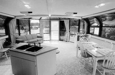
| Kitchen | 0.650 |  |
 |
 |
 |
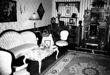
 LivingRoom |
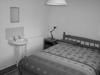
 Bedroom |
 LivingRoom |
 Bedroom |
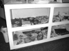
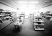
| Store | 0.730 |  |
 |
 |
 Industrial |
 Bedroom |
 Suburb |
 Industrial |
|
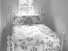
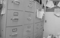
| Bedroom | 0.570 | 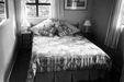 |
 |
 |
 |
 LivingRoom |
 OpenCountry |
 LivingRoom |
 Office |
| LivingRoom | 0.570 |  |
 |
 |
 |
 Bedroom |
 TallBuilding |
 Industrial |
 Store |
| Office | 0.900 | 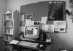 |
 |
 |
 |
 Kitchen |
 TallBuilding |
 Bedroom |
 Kitchen |
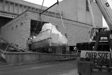
| Industrial | 0.580 | 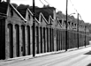 |
 |
 |
 Coast |
 Street |
 InsideCity |
 Mountain |
|
| Suburb | 0.990 |  |
 |
 |
 |
 Industrial |
 TallBuilding |
 Forest |
|
| InsideCity | 0.690 |  |
 |
 |
 |
 Store |
 Street |
 Industrial |
 Bedroom |
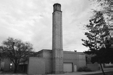
| TallBuilding | 0.800 |  |
 |
 |
 |
 Store |
 Street |
 Mountain |
 Industrial |
| Street | 0.810 |  |
 |
 |
 |
 Forest |
 TallBuilding |
 Highway |
 InsideCity |
| Highway | 0.830 |  |
 |
 |
 |
 Coast |
 OpenCountry |
 LivingRoom |
 Kitchen |
| OpenCountry | 0.680 |  |
 |
 |
 |
 Coast |
 Mountain |
 Mountain |
 Industrial |
| Coast | 0.750 |  |
 |
 |
 |
 OpenCountry |
 Highway |
 Mountain |
 Industrial |
| Mountain | 0.830 |  |
 |
 |
 |
 Forest |
TallBuilding |
 OpenCountry |
 Forest |
| Forest | 0.900 |  |
 |
 |
 |
 TallBuilding |
 Bedroom |
Mountain |
 OpenCountry |
| Category name | Accuracy | Sample training images | Sample true positives | False positives with true label | False negatives with wrong predicted label | ||||