Project 4 / Scene Recognition with Bag of Words
In this project, I implemented a couple of scene recognition algorithms, specifically nearest neighbors and linear SVM classifiers. For feature extraction, I used the tiny images and bag of SIFT representations. I also tuned my feature extractor and classifier hyperparameters by using a validation set, evaluated the chosen hyperparameters with cross-validation, and implemented the naive Bayes nearest neighbor classifier (NBNN).
Feature extraction
Tiny images
I resize each image to a 16-by-16 image, zero-center it, normalize it, and vectorize it.
function image_feats = get_tiny_images(image_paths)

N = length(image_paths);
img_size = 16;
d = img_size^2;

image_feats = zeros(N, d);
for i = 1:N
    img = imread(image_paths{i});
    img_resized = imresize(img, [img_size, img_size]);
    img_vector = double(img_resized(:));
    img_vector = img_vector - mean(img_vector);
    img_vector = img_vector / norm(img_vector);
    image_feats(i,:) = img_vector;
end
Bag of SIFT features
To make the bag of SIFT features feasible, I first compute a vocabulary of visual SIFT words. I compute all of the SIFT features from a training set of images and then run k-means clustering. The k returned centers are the k words for the vocabulary. The SIFT step parameter is set to 50 pixels to make sure the code runs quickly enough while still extracting enough SIFT features to have meaningful centers.
function vocab = build_vocabulary( image_paths, vocab_size, varargin )

sift_size = set_options({'sift_size'}, [3], varargin{:});
sift_step = 50;

all_sift_features = [];
for i = 1:length(image_paths)
    img = im2single(imread(image_paths{i}));
    [~, sift_features] = vl_dsift(img, 'step', sift_step, 'size', sift_size);
    all_sift_features = cat(2, all_sift_features, sift_features);

end
vocab = vl_kmeans(single(all_sift_features), vocab_size)';
With this vocabulary, I can extract a histogram feature from each image. The histogram contains as many bins as words in the vocabulary. The count in a bin is the number of times that corresponding word was the closest word to a SIFT feature. Within the code, I compute all the distances between the raw SIFT features and the visual words. For each SIFT feature, I find its closest word and increment the corresponding bin. After looping through all images, I normalize each histogram to prevent the number of SIFT features from influencing the extracted features.
function image_feats = get_bags_of_sifts(image_paths, varargin)

load('vocab.mat');
vocab_size = size(vocab, 1);
image_feats = zeros(length(image_paths), vocab_size);

[sift_step, sift_size] = set_options({'sift_step', 'sift_size'}, ...
    [10, 3], varargin{:});

for i = 1:length(image_paths)
    img = im2single(imread(image_paths{i}));
    [~, sift_features] = vl_dsift(img, 'step', sift_step, 'size', sift_size);
    D = vl_alldist2(single(sift_features), vocab');
    for j = 1:size(D, 1)
        [~, idx] = min(D(j,:));
        image_feats(i, idx) = image_feats(i, idx) + 1;
    end
    image_feats(i,:) = image_feats(i,:) / norm(image_feats(i,:));

end
Classification
1-nearest neighbor
I find all of the distances between the training features and the test features. I then iterate through each test image, setting its category to the one of the closest training feature.
function predicted_categories = nearest_neighbor_classify(train_image_feats, train_labels, test_image_feats)

[N, d] = size(train_image_feats);
M = size(test_image_feats, 1);
D = vl_alldist2(test_image_feats', train_image_feats');

predicted_categories = cell(M, 1);
for i = 1:M
    [~, idx] = min(D(i,:));
    predicted_categories{i} = train_labels{idx};
end
Linear SVM
For each category, I find the corresponding SVM using the 1-vs-all approach. I apply all the SVM's on the test features and categorize each one by the SVM that achieved the highest score.
function predicted_categories = svm_classify(train_image_feats, train_labels, test_image_feats, varargin)

lambda = set_options({'lambda'}, [0.0001], varargin{:});

W = zeros(size(train_image_feats,2), num_categories);
b = zeros(1, num_categories);
for i = 1:num_categories
    category = categories{i};
    labels = double(strcmp(category, train_labels));
    labels(labels == 0) = -1;
    [W(:,i), b(i)] = vl_svmtrain(train_image_feats', labels, lambda);
end

scores = bsxfun(@plus, test_image_feats*W, b);
[~, indices] = max(scores, [], 2);
predicted_categories = categories(indices);
Results on test set
After tuning the hyperparamters (see the validation section), I ran each classifier pipeline on the training and test sets. On top of measuring test accuracy, I measured the time to generate the vocabulary (if applicable) and the time thereafter to extract the features, train the classifier, and label the test data.
| 1-NN (tiny images) | 1-NN (bag of SIFT) | SVM | NBNN | |
| Test set accuracy | 22.5% | 53.1% | 62.7% | 62.8% |
| Vocab. time (min) | n/a | 1.9 | 3.8 | n/a |
| Pipeline time (min) | 0.1 | 8.9 | 8.6 | 6.5 |
The SVM and NBNN classifiers have nearly the same accuracy, with the NBNN classifier performing 0.1% better. One notable advantage of the NBNN classifier is that it doesn't need a vocabulary and runs two minutes faster on training and classifying (five minutes faster if we include the vocabulary generation).
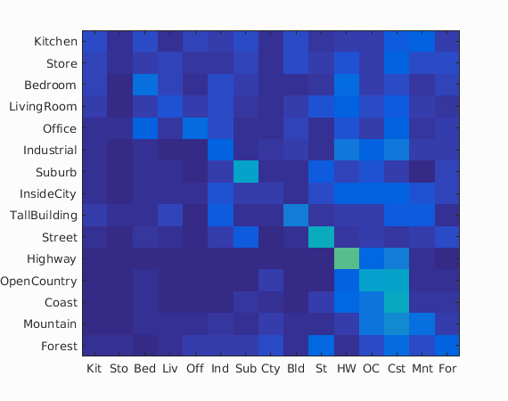
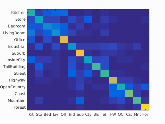
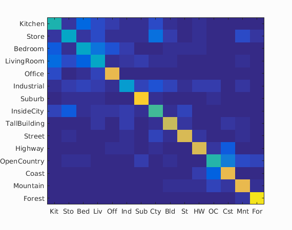
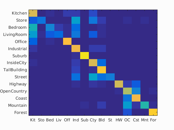
The above images are the confusion matrices (from left to right, 1-NN with tiny images, 1-NN with bag of SIFT features, linear SVM, and NBNN). The 1-NN classifier appears to improve across the board when using SIFT features, likely due to overfitting issues on the tiny images. Comparing the SVM and NBNN classifiers, it seems the NBNN is less "spread out" in that mistakes tend to pick among a small set of different images. The linear SVM, on the other hand, seems to pick more uniformly among other images when it makes a mistake.
Shown below is a larger confusion matrix for the NBNN along with more detailed information about its labelings of the test set.

Accuracy (mean of diagonal of confusion matrix) is 0.628
| Category name | Accuracy | Sample training images | Sample true positives | False positives with true label | False negatives with wrong predicted label | ||||
|---|---|---|---|---|---|---|---|---|---|
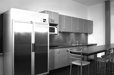
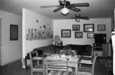
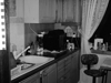
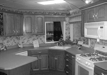
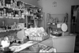
| Kitchen | 0.760 | 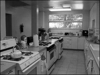 |
 |
 |
 |
 LivingRoom |
 LivingRoom |
 Industrial |
 InsideCity |
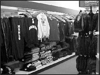
| Store | 0.200 | 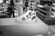 |
 |
 |
 |
 LivingRoom |
 Bedroom |
 Industrial |
 Kitchen |
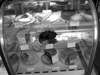
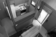
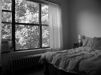
| Bedroom | 0.250 |  |
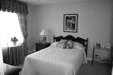 |
 |
 |
 Kitchen |
 LivingRoom |
 Kitchen |
 Industrial |
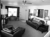
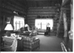
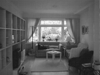
| LivingRoom | 0.160 |  |
 |
 |
 |
 Bedroom |
 Bedroom |
 Bedroom |
 Office |
| Office | 0.840 |  |
 |
 |
 |
 Kitchen |
 InsideCity |
 Kitchen |
 LivingRoom |
| Industrial | 0.810 |  |
 |
 |
 |
 Kitchen |
 Street |
 InsideCity |
 InsideCity |
| Suburb | 0.950 |  |
 |
 |
 |
 Highway |
 Mountain |
 Industrial |
 OpenCountry |
| InsideCity | 0.750 |  |
 |
 |
 |
 Bedroom |
 Street |
 TallBuilding |
 Industrial |
| TallBuilding | 0.870 |  |
 |
 |
 |
 Mountain |
 Bedroom |
 InsideCity |
 Industrial |
| Street | 0.230 |  |
 |
 |
 |
 Industrial |
 InsideCity |
||
| Highway | 0.740 |  |
 |
 |
 |
 OpenCountry |
 OpenCountry |
 Coast |
 OpenCountry |
| OpenCountry | 0.680 |  |
 |
 |
 |
 Highway |
 Forest |
 Coast |
 Coast |
| Coast | 0.810 |  |
 |
 |
 |
 OpenCountry |
 Mountain |
 OpenCountry |
 OpenCountry |
| Mountain | 0.480 |  |
 |
 |
 |
 TallBuilding |
 OpenCountry |
Suburb |
 OpenCountry |
| Forest | 0.890 |  |
 |
 |
 |
 OpenCountry |
 Mountain |
OpenCountry |
 OpenCountry |
| Category name | Accuracy | Sample training images | Sample true positives | False positives with true label | False negatives with wrong predicted label | ||||
Extra credit: Tuning hyperparameters with validation set
To properly tune the hyperparameters, I divided the original training set into a training set and validation set, each with 750 images (50 images per category). For the nearest neighbor and SVM classifiers, I then found the validation error over all combinations of the following hyperparameters:
- Vocabulary size: 10, 20, 50, 100, 200, 400, 1000, 10000 words
- SIFT bin size: 3, 5, 7, 9
- Steps per SIFT descriptor: 5, 10, 25, 50
- SVM L2 regularizer: 10-6, 10-5, 10-4, 10-3, 10-2, 10-1, 100
The graphs below show the best validation error achieved over each of the hyperparameter settings. The SVM doesn't appear to be majorly affected by the SIFT bin size, while the 1-NN seems to mostly lose performance with larger bin size (since "coarser" features may not be beneficial). For both classifiers, a larger SIFT step size makes performance suffer since the classifiers have less features to work with. For the SVM L2 regularizer, low values have approximately the same performance, while past a certain value the validation accuracy decreases due to the SVM prioritizing larger margins over number of errors.
Trading off for both accuracy and running time, I chose the following hyperparameters:
| Classifier | Vocab. size | SIFT size | SIFT steps | L2 regularizer | Validation accuracy |
| 1-NN | 100 | 3 | 5 | n/a | 43.2% |
| SVM | 100 | 9 | 10 | 10-4 | 57.3% |
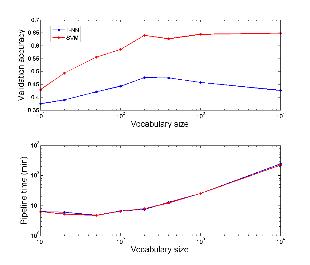
Extra credit: Vocabulary size
The plot below shows for each vocabulary size the best validation accuracy found for each classifier. The SVM consistently outperforms the nearest neighbor and doesn't overfit for large vocabulary size, instead flatlining. Large vocabulary sizes do also increase computation time, forcing smaller vocabulary sizes when the code is run end-to-end. In terms of accuracy, two hundred words appears to be the best choice. However, to ensure the code runs within ten minutes, I chose to use one hundred words.
Extra credit: Naive Bayes nearest neighbor
I also implemented the naive Bayes nearest neighbor classifier from this paper. Since finding the nearest neighbor would take too long, I used VLFeat's k-d tree implementation to perform approximate nearest neighbor search. With some tuning on both accuracy and speed, I set the number of comparisons in the nearest neighbor search to 100, the SIFT step size to 10 pixels, and the SIFT bin size to 3. With these hyperparameters, I achieved a 57.5% validation accuracy.
function predicted_categories = nbnn_classify(train_image_paths, train_labels, ...
    test_image_paths, varargin)

% Classifies images using the NBNN algorithm.

[sift_step, sift_size] = set_options({'sift_step', 'sift_size'}, ...
    [100, 3], varargin{:});

categories = unique(train_labels);
num_categories = length(categories);

disp('Extracting SIFT features for categories...');
category_features = extract_category_features(train_image_paths, train_labels, ...
    categories, sift_step, sift_size);
kd_trees = build_kd_trees(category_features);

disp('Extracting SIFT features from test images...');
[test_features, indices] = extract_features(test_image_paths, sift_step, sift_size);

disp('Classifying images...');
distances_to_categories = zeros(length(test_image_paths), num_categories);
for i = 1:num_categories
    [~, closest_distances] = vl_kdtreequery(kd_trees{i}, category_features{i}, ...
        test_features, 'maxnumcomparisons', 100);
    for j = 1:length(test_image_paths)
        distances_to_categories(j, i) = ...
            sum(closest_distances(indices(j):indices(j+1)-1));
    end
end
[~, indices] = min(distances_to_categories, [], 2);
predicted_categories = categories(indices);

end

function category_features = extract_category_features(image_paths, labels, ...
    categories, sift_step, sift_size)

category_features = cell(length(categories), 1);
for i = 1:length(categories)
    category_features{i} = [];
end

for i = 1:length(image_paths)
    img = im2single(imread(image_paths{i}));
    [~, img_sift_features] = vl_dsift(img, 'step', sift_step, 'size', sift_size);

    category_idx = find(strcmp(labels{i}, categories));
    category_features{category_idx} = cat(2, category_features{category_idx}, ...
        single(img_sift_features));

end

end

function kd_trees = build_kd_trees(sift_features)
% Builds a cell of KD trees, one for each SIFT feature cell.

kd_trees = cell(size(sift_features));
for i = 1:length(kd_trees)
    kd_trees{i} = vl_kdtreebuild(sift_features{i});
end

end

function [features, indices] = extract_features(image_paths, sift_step, sift_size)

features = [];
indices = zeros(length(image_paths)+1, 1);
indices(1) = 1;

for i = 1:length(image_paths)
    img = im2single(imread(image_paths{i}));
    [~, img_features] = vl_dsift(img, 'step', sift_step, 'size', sift_size);
    features = cat(2, features, single(img_features));
    indices(i+1) = size(features, 2) + 1; % index of next image
end

end
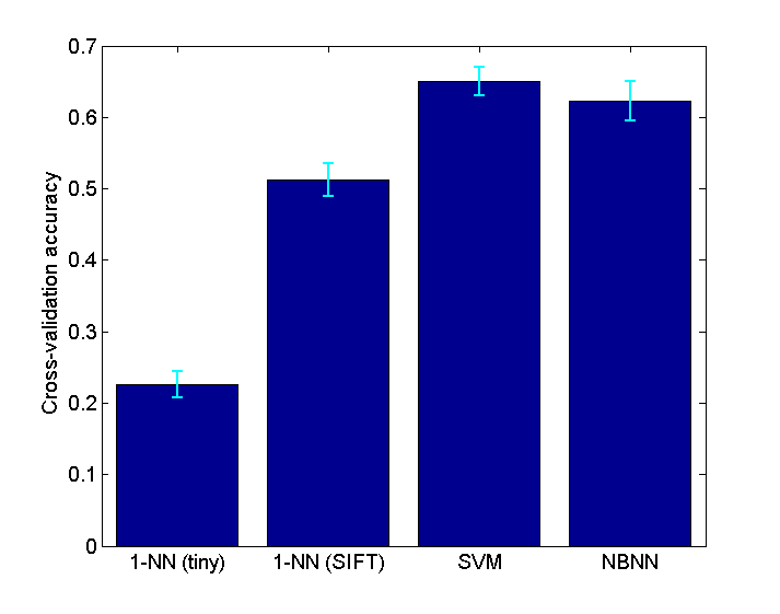
Extra credit: Cross-validation
To better evaluate the chosen hyperparameters, I also performed cross-validation. I merged both the training and test sets, and then I randomly sampled without replacement 100 images per category for each of the two sets. I then found the average and standard deviation in the accuracy over ten iterations. The averages and error bars (2 standard deviations on each side) are shown below.