Project 4 / Scene Recognition with Bag of Words
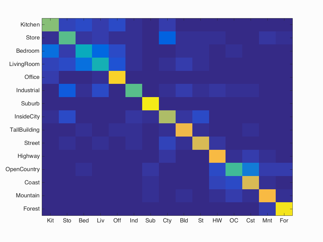
Confusion matrix of optimal results with accuracy of 70.3%.
Recognizing specific scenes, and what sort of environment they exist in is quite a common application of Computer Vision. The same methods used to identify certain scenes can often be extended to recognize objects within scenes, and as Professor Hays showed us earlier in the semester, can be used for results such as creating combination images that are a completely new scene built out of a variety of different scenes.
For this project, I implemented scene recognition using three combinations of methods as follows:
- Tiny image representations and nearest neighbor classifiers
- Bag of SIFT representations and nearest neighbor classifiers
- Bag of SIFT representation and linear SVM classifiers
Tiny Images and Nearest Neighbors
The "Tiny Image" feature is quite a simple image representation. It revolves around simply resizing the image, and adjusting its mean and unit length. Although resizing and modifying the images as so loses a large amount of the information encoded in the image (such as high frequency content) we did not worry too much about that in this phase of the project because this was simply a baseline.
The Nearest Neighbor classifier is a well known classifier in Machine Learning that is focused on the idea that the closest "neighbor" to a value has a reasonable likelihood to have the same classification. It is traditionally used in a K-Nearest Neighbors setup where the K nearest values to the one being classified "vote" on the classification of the value. In my implementation of the Nearest Neighbor classifier, I experimented with different values for K, but found that the best results came from using the single nearest neighbor to the image being classified, which gave me the highest accuracy of 22.5% (not great, but its a start). My results for different values of K are shown below:
| K Value | 1 | 5 | 10 | 15 | 20 |
| Accuracy | 22.5% | 21.5% | 21.3% | 22.1% | 22.2% |
As you can observe, increasing the number of neighbors used to classify images did not provide a meaningful effect on the accuracy of the classifications in this portion of the project, and for this reason, I used the single nearest neighbor to classify images.
Bag of SIFT and Nearest Neighbors
The second portion of this project focused on using bags of quantized SIFT features to represent our images. This concept is focused on the idea of establishing a "vocabulary" of visual words that are formed from sampling features of our training set and then clustering them using kmeans. I experimented with using different SIFT step sizes when creating the vocabularies and recoginzed that since we were using SIFT, the step size was one be considered when clustering words, as too large of steps would lose information, and too small of steps would risk overfitting the images. I settled for a step size of 8, after testing with step sizes of 4 and 10 for my vocabulary, as this gave me a reasonable level of accuracy.
Once the vocabulary was created, it was now time to create the bags of SIFT descriptors for our images. This was accomplished by sampling SIFT descriptors and clustering them into the categories created by our vocabulary. By doing this, we were able to create a histogram of bins where each bin counted how many times a SIFT descriptor was assigned to a certain cluster. This again required tweaking the step sizes used in the SIFT sampling, which will be discussed more later on.
This portion of the project still used the same Nearest Neighbor classifier used in part one of the project, so I will not describe it again in depth. My results below are based on varying the step distances in selecting features for the bags. I did not vary the number of neighbors, as the first part of our project showed that differing numbers of neighbors had little difference on similar inputs of this nature. My results for different step sizes are shown below:
| Step Size | 1 | 2 | 4 | 8 | 12 |
| Accuracy | 54.5% | 54.3% | 53.5% | 53.1% | 48.7% |
Predictably, smaller step sizes led to better accuracy since smaller amounts of pixels were being considered at a time. While the smaller step sizes provided minor accuracy improvements, they greatly increased the amount of computation time due to the greater number of computations needed to carry out the analysis. To put it in perspective, step sizes of 1 and 2 took 45 and 14 minutes to run on my machine, respectively. In contrast, running this setup with a step size of 4 took 6 minutes, and was able to classify images with only a 1% loss of accuracy. Due to this, I decided to move forward with a step size of 4, as it represented an even trade off between computing time and accuracy.
Bag of SIFT and Linear Support Vector Machines
The final portion of this projects focused on taking the bags of visual words that we created using SIFT and use them to create linear SVM classifiers to determine what scene different images belonged to. Since I previously described the general idea behind Bags of SIFT features, I will not go into anymore depth, I will simply add that I continued to use a step size of 4 based on the results of the previous portion.
The addition to this portion of the project was using Linear Support Vector Machines as classifiers for our images. Linear Support Machines work as classifiers by representing a feature space partitioned by a learned hyperplane, and images being classified by which side of that hyperplane they fall on, one side being a match, and the other being a mis-match. These SVM classifiers were tuned by changing the lambda parameter, which is a value that determines the range formed around the hyperplane separator to classify objects. The idea is based on a higher lambda value leading to a smaller range of values that can be classified as correct. Based on this, I experimented with different values of lambda for my Linear SVM Classifier. My results for different lambda values are shown below:
| Lambda | 0.000001 | 0.00001 | 0.0001 | 0.001 | 0.01 | 0.1 |
| Accuracy | 64.5% | 67.3% | 70.3% | 61.3% | 45.1% | 48.9% |
Due to the nature of the lambda parameter, as lambda becomes larger, less and less wrongly classified examples will occur since the classifier is becoming more and more specific. As the data shows, increasing the size of lambda did improve the accuracy of the classifier, up to a certain extent. The data actually exhibited a peak, with the most accurate classification coming from a lambda of 0.0001. Once lambda was increased past that boundary, the accuracy began decreasing again, most likely because the larger lambda was constraining the classifier too much, and overfitting the training data, leading to decreased accuracy
The following images are my confusion matrix and some sample results of my scene recognizer after tuning it to the most accurate level I could achieve (70.3% correct matches). This accuracy level was achieved with the following parameters.
| Lambda | Bag of SIFT step size | Vocabulary step size | Vocabulary size | Accuracy | Runtime |
| 0.0001 | 4 | 8 | 200 | 70.3% | 328 seconds (5.46 minutes) |
Scene classification results visualization
Accuracy (mean of diagonal of confusion matrix) is 0.703
| Category name | Accuracy | Sample training images | Sample true positives | False positives with true label | False negatives with wrong predicted label | ||||
|---|---|---|---|---|---|---|---|---|---|
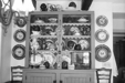
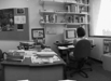
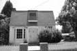
| Kitchen | 0.610 |  |
 |
 |
 |
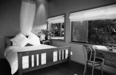
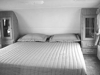
 Bedroom |
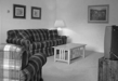
 LivingRoom |
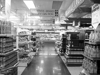
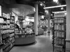
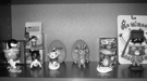
 Store |
 TallBuilding |
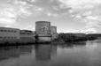
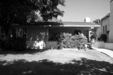
| Store | 0.560 |  |
 |
 |
 |
 InsideCity |
 Industrial |
 InsideCity |
 Street |
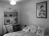
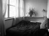
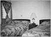
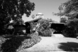
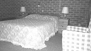
| Bedroom | 0.410 |  |
 |
 |
 |
 Store |
 LivingRoom |
 OpenCountry |
 Street |
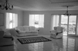
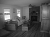
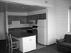
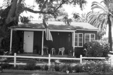
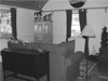
| LivingRoom | 0.450 | 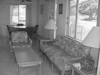 |
 |
 |
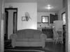 |
 Kitchen |
 Street |
Bedroom |
 Office |
| Office | 0.900 | 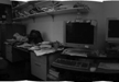 |
 |
 |
 |
 Kitchen |
 Bedroom |
 LivingRoom |
 Kitchen |
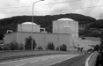
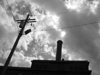
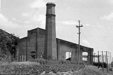
| Industrial | 0.560 |  |
 |
 |
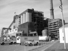 |
 Street |
 Suburb |
 Coast |
 Highway |
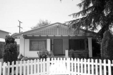
| Suburb | 0.960 | 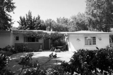 |
 |
 |
 |
 Mountain |
 OpenCountry |
 Street |
Industrial |
| InsideCity | 0.680 |  |
 |
 |
 |
 Store |
 TallBuilding |
 Store |
 Street |
| TallBuilding | 0.810 |  |
 |
 |
 |
 LivingRoom |
 Street |
 Street |
 Industrial |
| Street | 0.750 |  |
 |
 |
 |
 Industrial |
Bedroom |
 Store |
 Industrial |
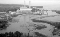
| Highway | 0.820 |  |
 |
 |
 |
 Mountain |
 Street |
 Coast |
 Coast |
| OpenCountry | 0.520 |  |
 |
 |
 |
 Bedroom |
 Coast |
 Coast |
 Highway |
| Coast | 0.760 |  |
 |
 |
 |
OpenCountry |
 OpenCountry |
 OpenCountry |
 Highway |
| Mountain | 0.820 |  |
 |
 |
 |
 Forest |
 Highway |
 TallBuilding |
 LivingRoom |
| Forest | 0.940 |  |
 |
 |
 |
 Mountain |
 Industrial |
 Mountain |
 Industrial |
| Category name | Accuracy | Sample training images | Sample true positives | False positives with true label | False negatives with wrong predicted label | ||||
General Results, and Parameters
The following tables contain my configurations for the optimal results I was able to achieve by tuning the different portions of this project
Tiny Images and Nearest Neighbors
| K neighbors | Accuracy | Runtime |
| 1 | 22.5% | 19 seconds |
Bag of Sift and Nearest Neighbors
| SIFT Bag Step Size | SIFT Vocab Step Size | Vocab Size | K neighbors | Accuracy | Runtime |
| 4 | 8 | 200 | 1 | 53.5% | 347 seconds (5.78 minutes) |
Bag of Sift and Linear Support Vector Machine
| SIFT Bag Step Size | SIFT Vocab Step Size | Vocab Size | Lambda | Accuracy | Runtime |
| 4 | 8 | 200 | 0.0001 | 70.3% | 328 seconds (5.46 minutes) |