Project 4: Scene Recognition with Bag of Words
In this project, we will implement basic image recognition. The goal of the project is to be able to accurately classify a given image into one of 15 scenes that our classifier is trained on. We will start with a simple Bag of Words representation with a Nearest Neighbour classifier but will slowly work our way towards the more sophiticated stuff - Support Vector Machines for classification and a number of techniques for improving accuracy.
Base Model
In this base model, we will implement the following (in order)
- A nearest neighbour classifier with a tiny image feature representation
- A nearest neighbour classifier with a bag of sift feature representation
- A support vector machine classifier with a bag of sift feature representation
Free Parameter values
For the baseline model, we have chosen the size of the vocabulary to be 200 (inspired by the spatial pyramid paper). We like this value becuase the program execution does not take very long and it is sufficiently big to be useful as vocabulary size. While building the vocabulary, the step size is 10. While extracting features, the step size is 6. We find that this step size gives us good SIFT features in reasonable amount of time. Indeed, it takes ~240 seconds to extract features for a vocabulary size of 200. We do not subsample from the SIFT vectors; we use all of them. We have used the fast approximation of SIFT features everywhere since the slower version takes too long to execute.
Nearest Neighbour with Tiny Images
We implemented a tiny image representation for features and used a nearest neighbour classifier to classify the data. A tiny image representation resizes each image to a fixed resolution, which is fast but loses out on image information. A nearest neighbour classifier finds the nearest training example for each testing example.
When we use 1NN (searching for the nearest neighbour), we get an accuracy of 22.8%. That is much better the accuracy of a random classifier, which was 7%. Moreover, the entire program runs in 15.950532 seconds, which really speaks to the speed at which tiny images can be generated. Thus, we see first hand that tiny images, while not being very good respresentations of the information are very useful for running and testing algorithms on large datasets to get a baseline performance.
Nearest Neighbour with Bag of SIFT
We extend the bag of words model to images to form the bag of SIFT model. Here, the vocabulary conssists of SIFT features that are obtained by clustering over the SIFT feature space. We use this with a nearest neighbour classifier.
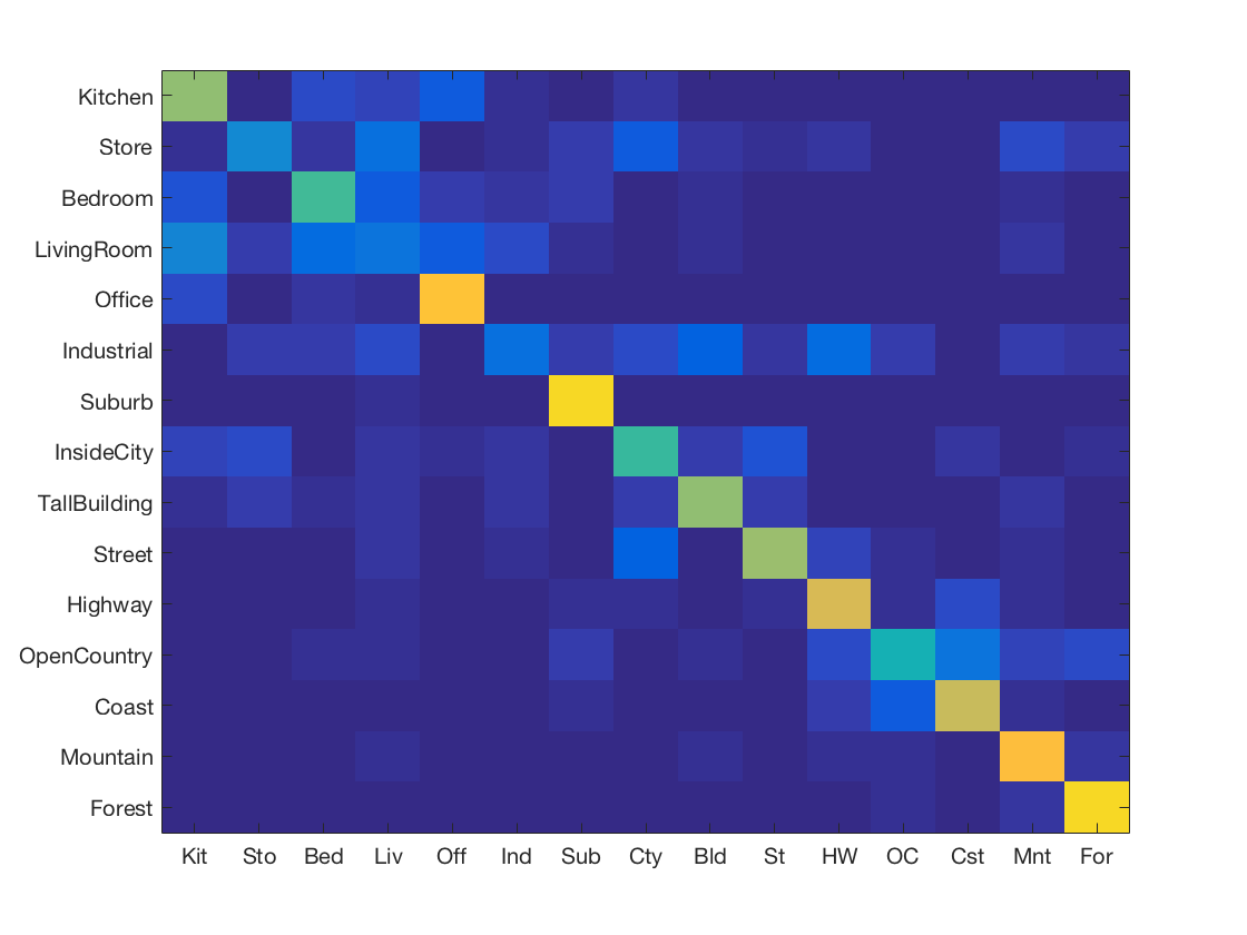
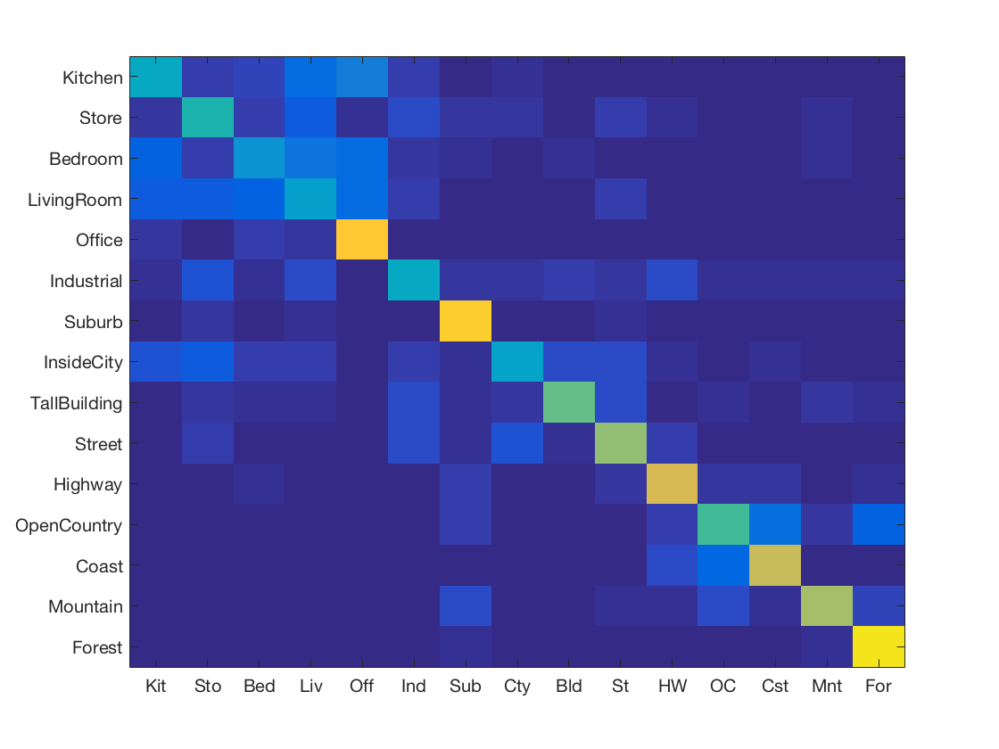
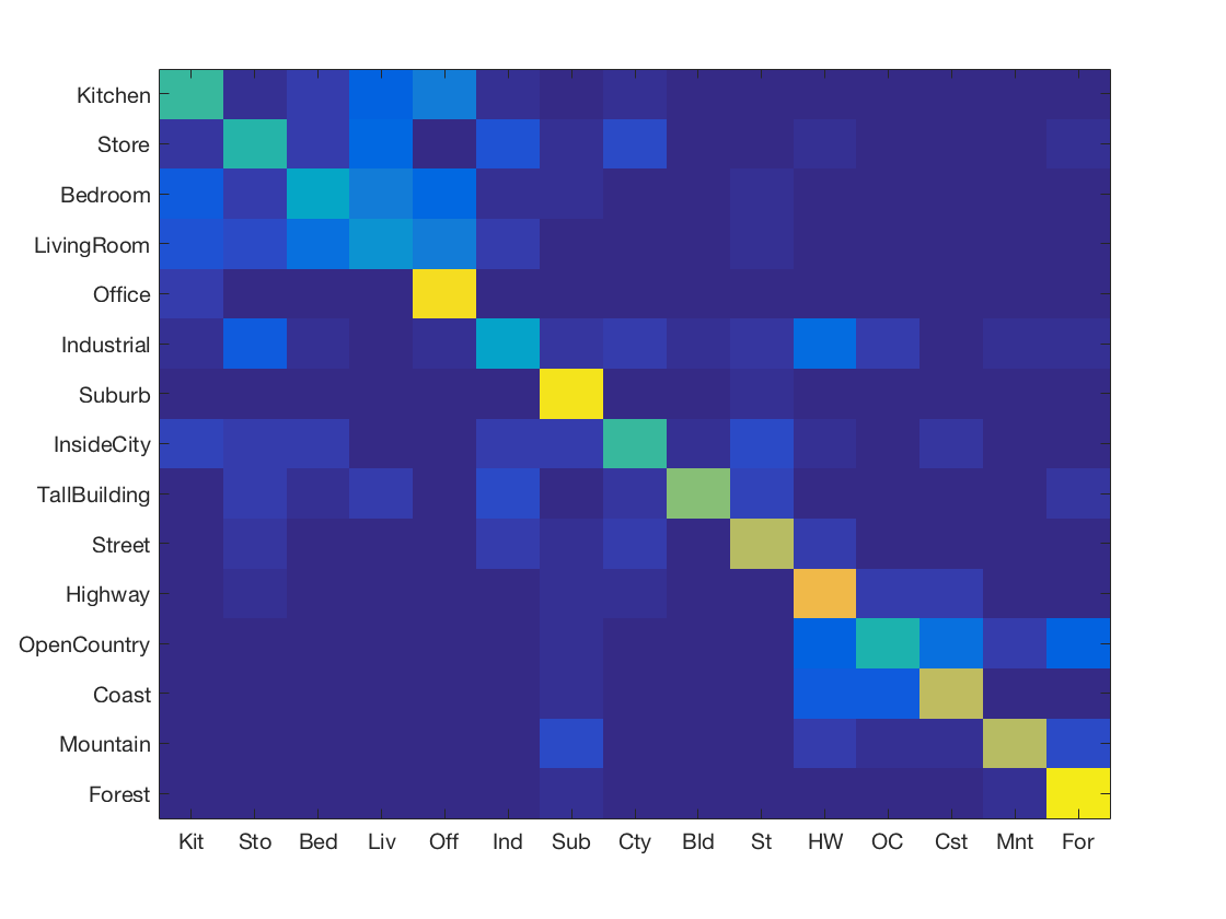
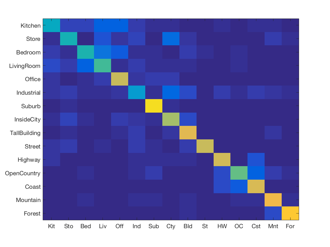
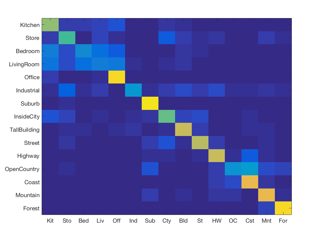
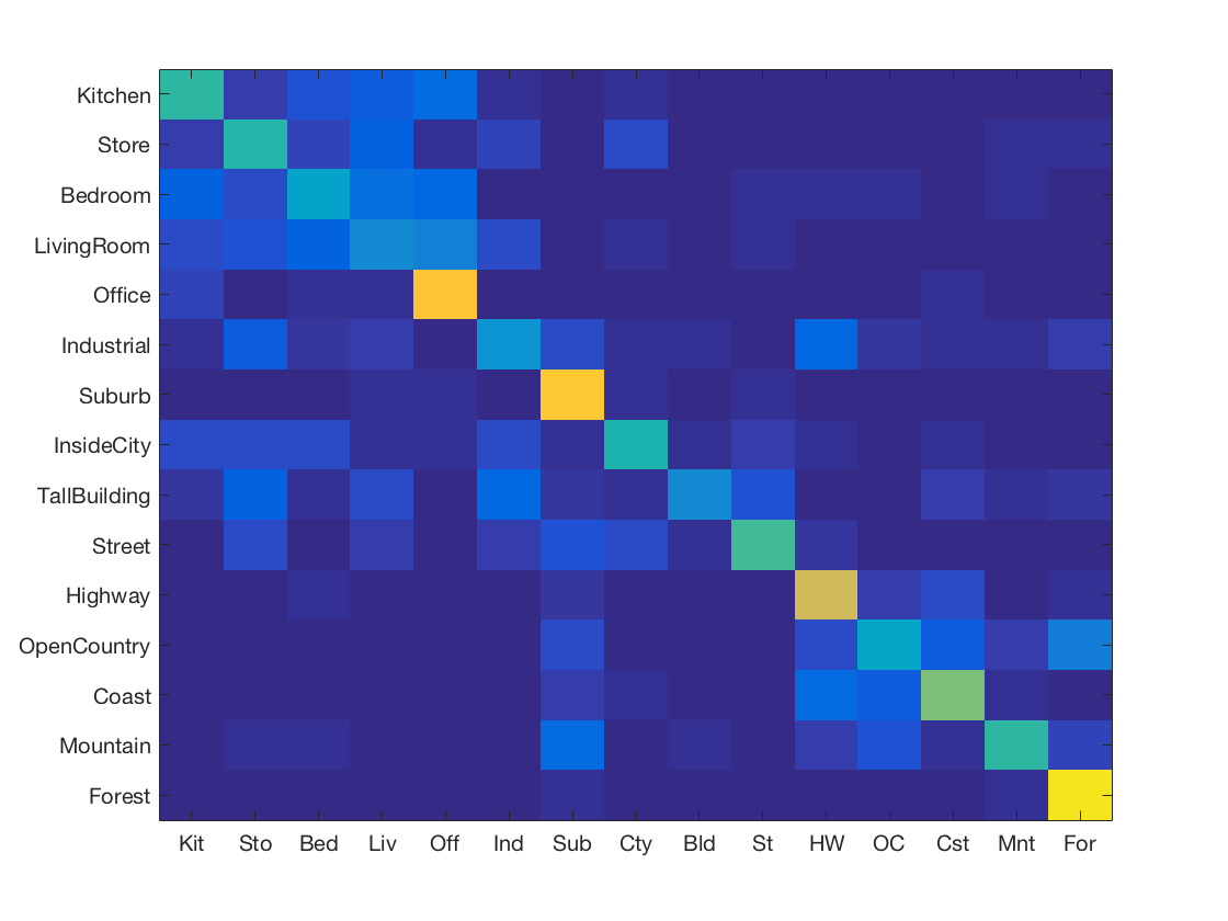
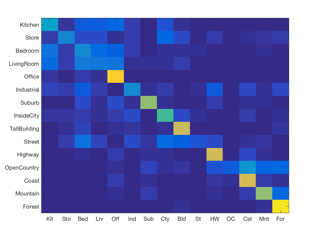
When we use 1NN (searching for the nearest neighbour), we get an accuracy of 52.8%. The entire code takes 479.595565 seconds to run (inclusing SIFT feature extraction). The confusion matrix is given below.
The confusion matrix shows us that the classifier has more trouble with the classes like Kitchen, Bedroom, Living Room, etc. However, it can classify Offices, Suburbs, Forests really well. At this point, we are not sure if the nearest neighbour algorithm is biased or if it is genuinely hard to classify those classes.
SVM with Bag of SIFT
We finally use a Support Vector Machine on our Bag of SIFT representation. The SVM gives us superior classification as compared to the nearest neighbour method.
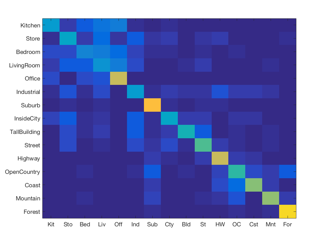
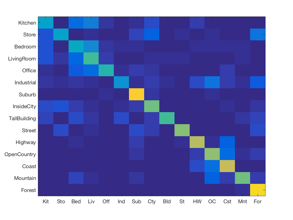
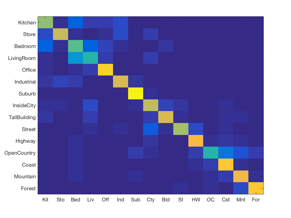
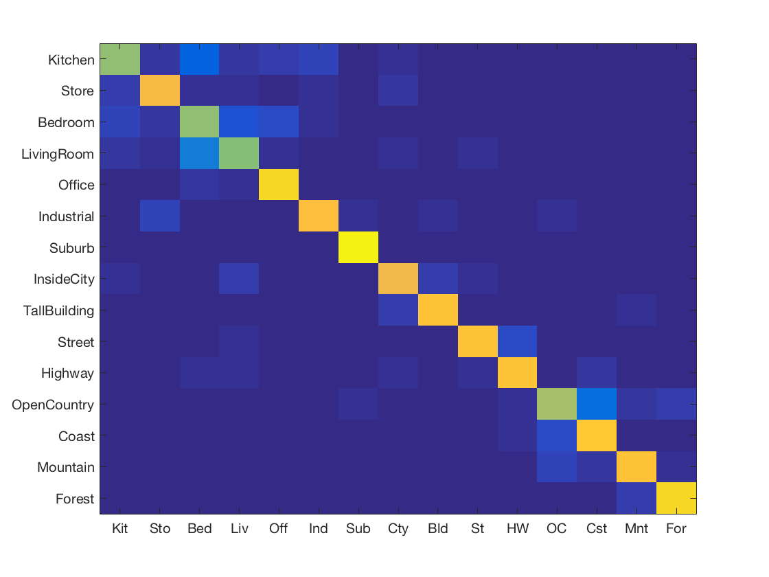
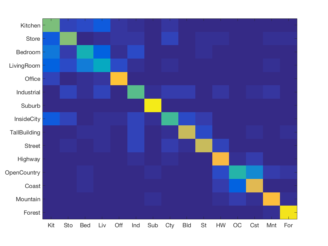
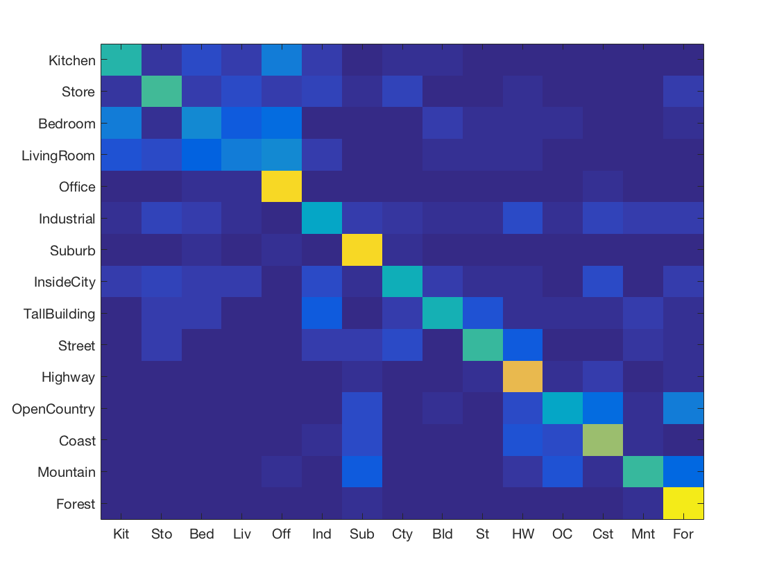
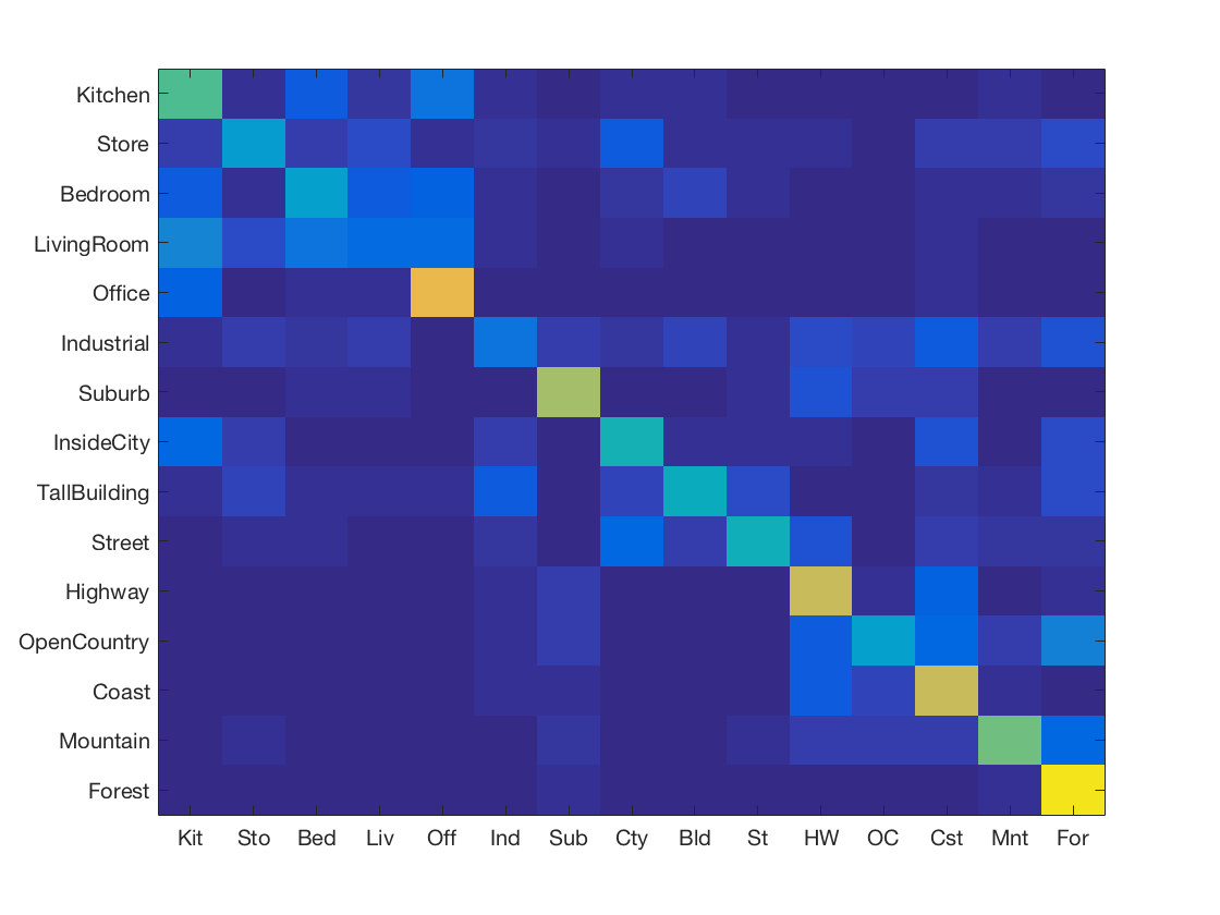
We obtain an accuracy of 67.2% using the SVM. The entire code takes 451.903990 seconds to run (including SIFT feature extraction). The confusion matrix is given below.
The confusion matrix shows us that the classifier has more trouble with the classes like Kitchen, Bedroom, Living Room, etc. However, it can classify Offices, Suburbs, Forests really well. This is similar to what we observed in the nearest neighbour classifier, so it must be harder to classify those classes.
We tried different values for lambda to arrive at the value that gave us the best result. The range of the order of magnitude for lambda experimented with was 0.00001 to 1.0. We found (not surprisingly) that regularization works well in tuning the SVM, however excessive regularization would hurt accuracy. The optimum value of lambda was determined to be 0.0001.
The nearest neighbour and SVM classifiers take about the same amount of time to run overall. On further inspection, we see that classifcation does not take a lot of time. Indeed, the bottle neck is computing the Bag of SIFT feature vector. Classification is speedy. As noted above, it takes about ~240 seconds to compute the Bag of SIFT feature description.
Improving the Baseline
The baseline model gives us good results for our classifier. However, we can improve upon this model using a number of techniques. We describe the techniques used and their impact on accuracy below.
We have also used Cross Validation to measure the performance of our algorithms. We take the average of ten randomly sampled training and test sets of size 100 each. We will report CV accuracy in addition to the fixed training and test set accuracy.
Nearest Neighbour - Chi Squared distance
A nearest neighbour algorithm depends highly on the distance metric used for determining relative closeness. We found that using the Chi Squared distance metric improves the accuracy of our algorithm. Running the same experiment as above, we get an accuracy of 59% for nearest neighbour with Chi Square. We get a ~7% boost in accuracy. CV Accuracy is 58.76%.
Nearest Neighbour - KNN
We can also use KNN, where we take the most popular category chosen by K nearest neighbours. Note that finding the most optimum value for K is an optimization problem. We experimentally determine this value. We tired different values of K (numbers from 1-11) and found K=7 to be the most optimal value.
Running K=7 on the Bag of Words representation gives us an accuracy of 54.6%. That gives us a 2% boost in accuracy. CV accuracy is 54.71%.
Nearest Neighbour - KNN with Chi Squared distance
We combine the above two methods. The accuracy is 62.4%. This combines the best of the above two methods. CV accuracy is 62.11%.
Feature Representation - Gist
The Gist descriptor is one of the methods of representing an image. It is a low dimensional representation that is based on local information. It is very useful and as we will see, is highly discriminative. We have used the descriptor with our classification methods. We have used it alone and in conjunction with SIFT.
Gist only
We get the following accuracies for our Gist descriptor in isolation
- 1NN - 51.5% [CV - 50.9%]
- KNN - 57.5% (K=8 optimal here) [CV - 57.48%]
- KNN with Chi Squared - 55.9% (K=7 optimal here) [CV - 55.75%]
- SVM - 64.9% (lambda=0.0001) [CV - 65.12%]
Thus, we see Chi-Squared distance does not work well for Gist. However, it still performs better than our improved KNN classifier that had only SIFT features. Interestingly, the SVM on only Gist gets an accuracy lesser than our SVM on only SIFT. However, the descriptor has low dimensionality, so it is commendable that it is still able to get a comparable performance.
SIFT + Gist
We get the following accuracies for our combined SIFT and Gist descriptor
- 1NN - 59.5% [CV - 58.95%]
- KNN - 63.9% (K=9 optimal here) [CV - 63.66%]
- KNN with Chi Squared - 68.7% (K=9 optimal here) [CV - 67.54%]
- SVM - 75.2% (lambda=0.0001) [CV - 76.1%]
Thus, we see that adding the Gist descriptor to our feature greatly enhances our classification capabilities. We see a boost of almost ~7% in our classification capabilities. We also see that Chi Squared distance works well with the combined feature even though it didn't work as well with Gist individually. This is likely because the number of dimensions of the SIFT descriptor exceed that of the Gist descriptor, so the overall descriptor is sensitive to the Chi-Squared distance metric.
Feature Quantization - Fisher
Up till now, we had been using the bag of SIFT model, that was based on a vocabulary of SIFT features. The vocabulary was created by applying a clustering algorithm (in this case KMeans) to the space of sampled SIFT descriptors. The number of clusters corresponded to the size of the vocabulary (200 in our case). Now, we will instead use another method to find the number of clusters. We will find them by fitting a Gaussian Mixture model to the data. Thus, it goes beyond the Bag of words model by capturing more than just count statistics. Moreover, instead of using SIFT descriptors on this data, we will use a Fisher vector, which gives better results.
Fisher only
We get the following accuracies for our Fisher descriptor in isolation
- 1NN - 46.7% [CV - 45.9%]
- KNN - 52.3% (K=9 optimal here) [CV - 51.22%]
- SVM - 73.5% (lambda=0.0001) [CV - 72.42%]
Although our KNN learner does moderately okay on the Fisher descriptor, the SVM does pretty good on the fisher vector in isolation. It'll be interesting to see how a combination of Fisher and Gist does, as they've been the best individual predictors.
Fisher + Gist
We get the following accuracies for our combined Fisher and Gist descriptor
- 1NN - 60.5% [CV - 60.54%]
- KNN - 64.7% (K=7 optimal here) [CV - 63.66%]
- SVM - 80.2% (lambda=0.00015) [CV - 79.45%]
Thus, we see that the fisher and gist combined feature vector gives us a very high degree of accuracy. Our KNN gets almost as much as the baseline SVM. Our SVM touches the 80% accuracy for the first time! Fisher and Gist, thus are very accurate.
Experimental Design - Vocbulary Size
We will use different vocabulary sizes for our Bag of SIFT representation and see how various algorithms perform on them. We will compare the 1NN learner, KNN Learner and SVM classifiers. What we expect to see is that our SVM wil outperform our KNN, which will outperform the 1NN learner. This experiment should be indicative of how vocabulary size affects the accuracy of the classifier. It helps answer the question, should we spend resources on creating and maintaing large vocabularies or do we reach the point of diminishing returns and it'd be better to focus our resources elsewhere. Other free parameters are as determined above.
Vocabulary Size vs Accuracy
The following table shows accuracy of the classifiers for various vocabulary sizes. The CV accuracy is given in angular brackets ([]).
|
M |
1NN |
KNN |
SVM |
|
50 |
49.7% [48.75%] |
52.6% [53.05%] |
61.1% [59.5%] |
|
100 |
53.1% [52.78%] |
53.6% [53.25%] |
62.4% [62.95%] |
|
200 |
52.8% [51.91%] |
54.6% [54.71%] |
67.2% [66.9%] |
|
500 |
54.7% [53.3%] |
55.6% [55.45%] |
68.8% [69.2%] |
|
1000 |
53.1% [53.2%] |
55.9% [55.75%] |
69.4% [69.5%] |
Thus, we see that increasing the size of the vocabulary gives us better results on average. Our SVM results are increasing monotonically as we go from 50 to 1000. However, for our 1NN classifier, a vocabulary size of 1000 is worse of than a size of 500. Moreover, the increase in accurcy as we increase the size of our vocabulary starts to slow down after 500. As we double the size from 500 to 1000, we get a lesser boost than what we got from 200 to 500. Thus, increasing the size of the vocabulary helps, but only so much. We have to look towards other methods from boosting our accuracy.
Best Results
Here, we display the best baseline and improved results.
Baseline
We get our best results with SVM. The accuracy is 67.9%.
Improved
We get our best results with SVM using Fisher and Gist descriptors. The accuracy is 80.3%
Feature Quantization - Soft Encoding
In soft encoding, we construct the histogram for our bag of SIFT features by making every point affect more than one cluster center based on their distance from them. This is thus a relaxation of the encoding algorithm, hence called soft encoding.
We get the following accuracies for our soft encoded bag of SIFT descriptors
- 1NN - 40.2% [CV - 40.1%]
- KNN - 42.8% (K=7 optimal here) [CV - 42.12%]
- SVM - 52.5% (lambda=0.0001) [CV - 52.32%]
Thus, we see that the results we get aren't better off than our baseline results.
Spatial Pyramid - Representation
In the spatial pyramid representation, we form a feature vector by recursively sub-dividing the image into halves and taking into account the SIFT features that are located only within the confines of the sub-divided image. This helps us oversome some of the spatial information we lose by converting an image to its bag of SIFTS representation as this representation is calculated at different levels of granularity.
We get the following accuracies for our Fisher descriptor in isolation
- 1NN - 51.3% [CV - 50.62%]
- KNN - 51.3% (K=7 optimal here) [CV - 51.0%]
- SVM - 60.5% (lambda=0.0001) [CV - 58.75%]
Thus, we see that the results we get very similar to our baseline results. We may not be taking complete advantage of this feature representation as we are not using the Pyramid matching kernel. If we use that, we should see a boost in accuracy.
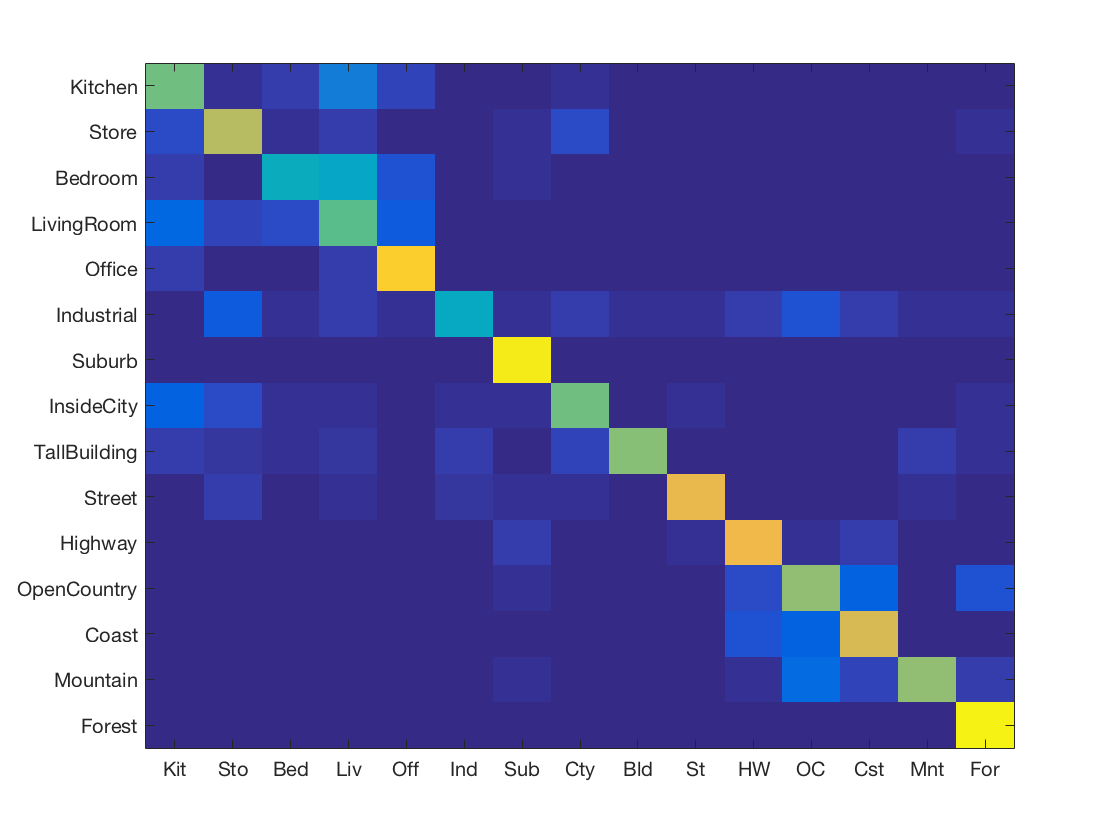
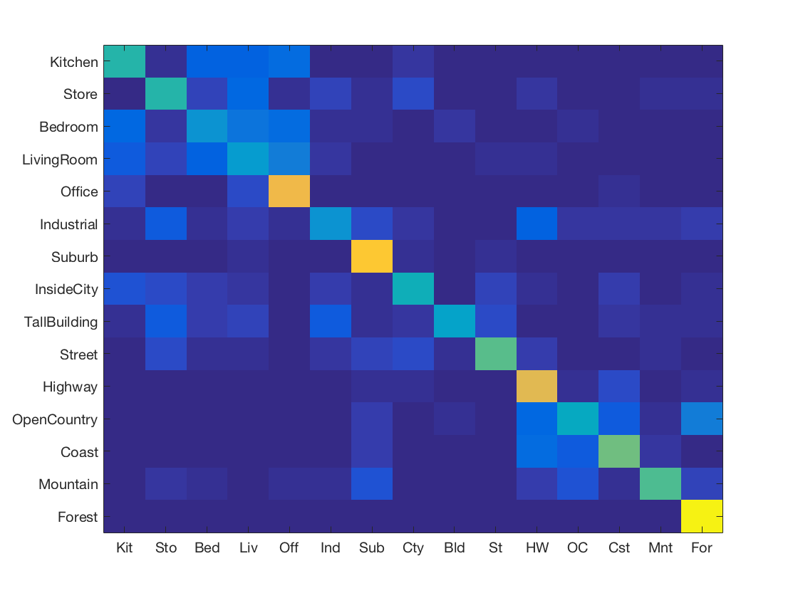
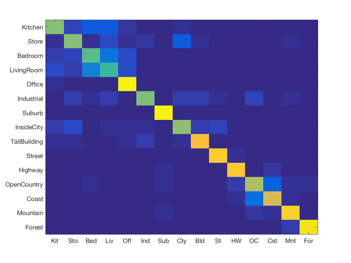
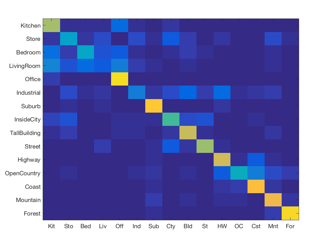
Confusion Matrices
Here, we will present labeled confusion matrices.
-
1 Nearest Neighbour using SIFT features with Chi Squared distance metric
-
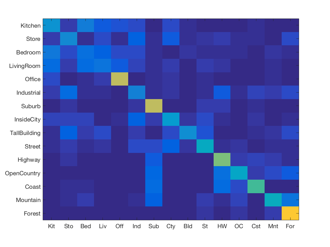
K Nearest Neighbours using Gist features
-
K Nearest Neighbours using SIFT + Gist features with Chi Squared distance metric
-
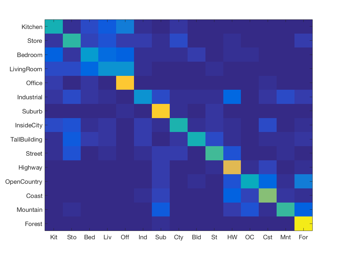
K Nearest Neighbours using SIFT features
-
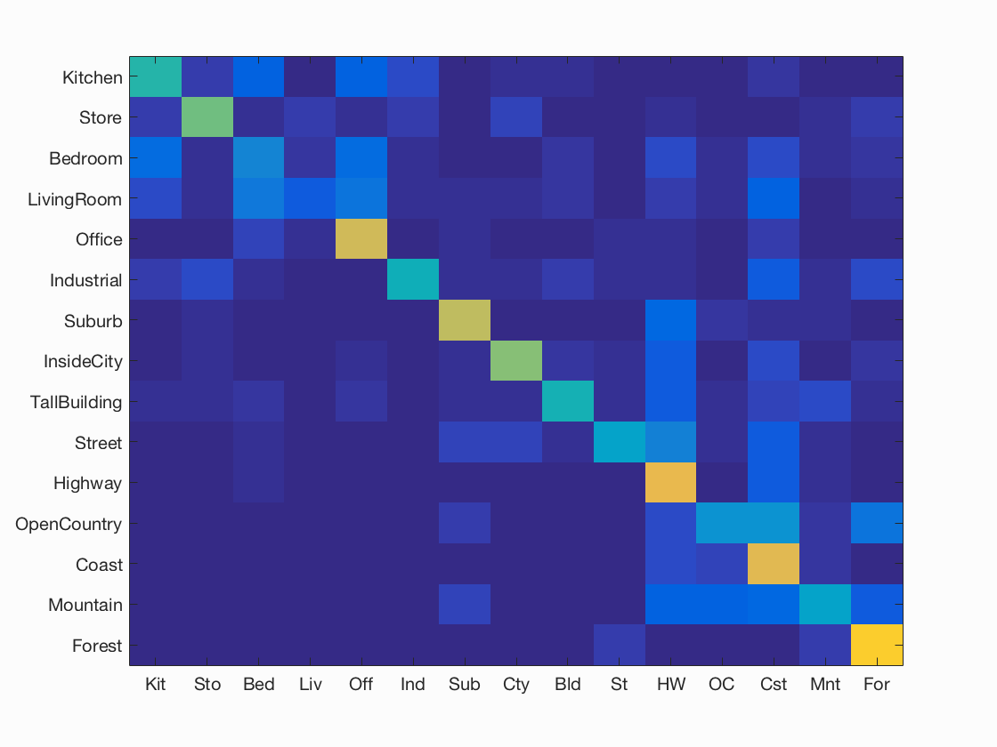
K Nearest Neighbours using SIFT features with Chi Squared distance metric
-
K Nearest Neighbours using Fisher vector
-
K Nearest Neighbours using Fisher vector + Gist
-
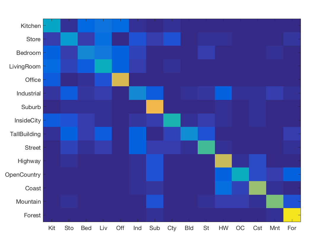
Support Vector Machine using Fisher vector
-
Support Vector Machine using Gist features
-
Support Vector Machine using Fisher vector + Gist
-
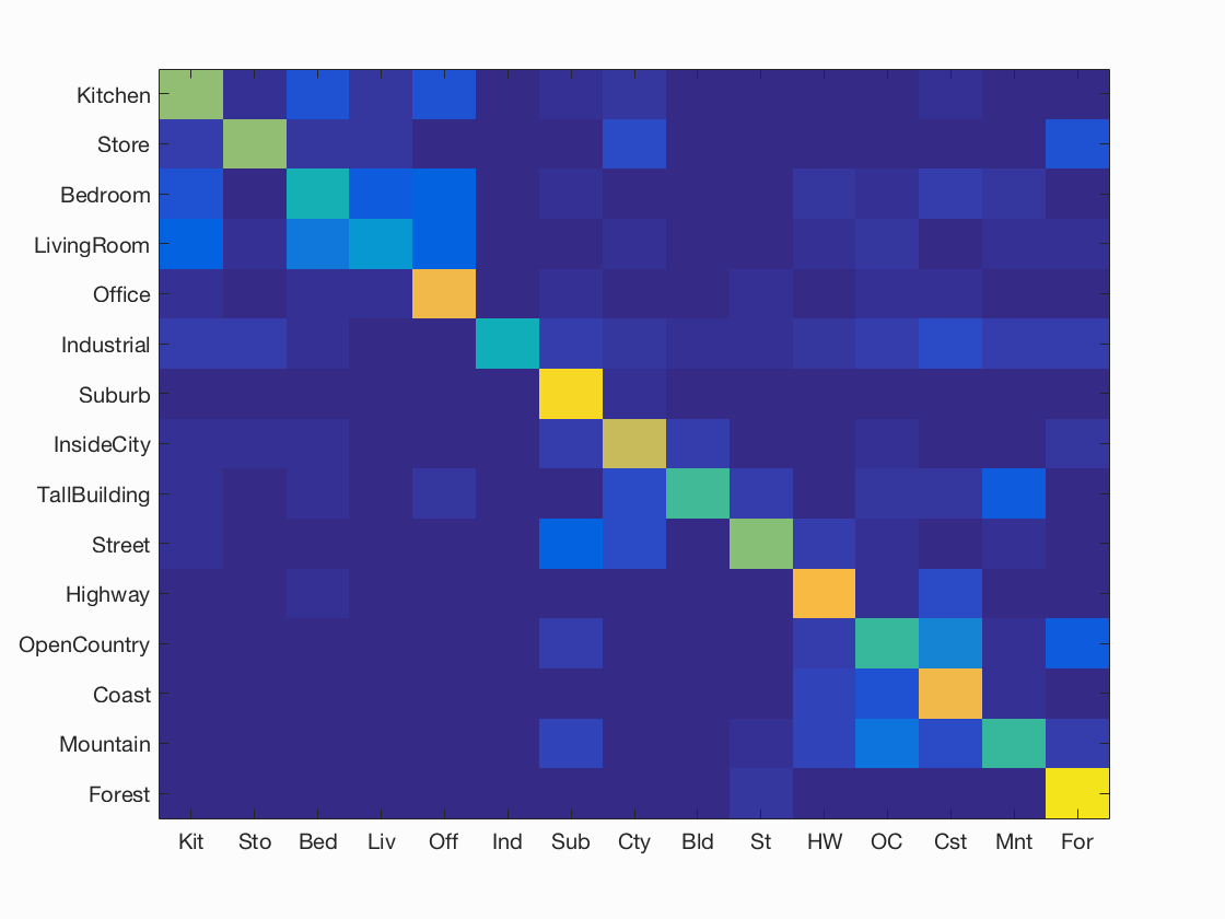
Support Vector Machine using SIFT + Gist features
-
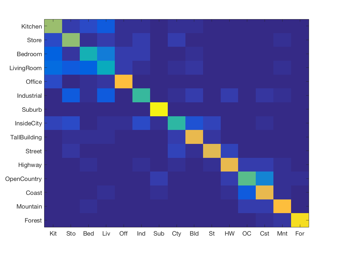
Support Vector Machine with SIFT and vocabulary size 50
-
Support Vector Machine with SIFT and vocabulary size 100
-
Support Vector Machine with SIFT and vocabulary size 200
-
Support Vector Machine with SIFT and vocabulary size 500
-
Support Vector Machine with SIFT and vocabulary size 1000
-
K Nearest Neighbours with SIFT and vocabulary size 50
-
K Nearest Neighbours with SIFT and vocabulary size 100
-
K Nearest Neighbours with SIFT and vocabulary size 200
-
K Nearest Neighbours with SIFT and vocabulary size 500
-
K Nearest Neighbours with SIFT and vocabulary size 1000
-
K Nearest Neighbours with SIFT and soft encoding
-
Support Vector Machine with SIFT and soft encoding
-
K Nearest Neighbours with SIFT and Spatial Pyramids
-
Support Vector Machine with SIFT and Spatial Pyramids