Robert Borowicz

Project 4 / Scene Recognition with Bag of Words

Contents

Example evaluation image

• Algorithm Explanation
• Build Vocabulary
• Tiny Images
• Nearest Neighbor Classifier
• Bag of Words
• Linear SVM Classifier
• Results
• Best Results
• Submitted Results
• Confusion Matrices

This project focused on scene recognition from a bag of words model. Below, I discuss the design of my algorithms, as well as discuss the different parameters that affected the final accuracy of the classifiers.

Algorithm Explanation

In order to achieve the best results, we have to first build a vocabulary.

Build Vocabulary

In order to build the vocabulary, we need to extract a large amount of SIFT features from many training images. The overall algorithm is quite simple. For every image, we first compute SIFT features and store all of these features in one large matrix. After this, we run vl_kmeans on these features, and specify our number of clusters, which in this case was 200. This gives us our 200 clustered centroids. This has dimension 128 x 200, so we transpose this to get our final vocabulary of dimension 200 x 128.

% We do this for all input images
[~, SIFT_feats] = vl_dsift(img, 'Step', 5, 'Fast');
all_SIFT_features = [all_SIFT_features SIFT_feats];

% Then we can cluster the SIFT features
[centroids, ~] = vl_kmeans(single(all_SIFT_features), vocab_size);

The vocab size, in this case 200, can be varied; although I chose not to for these tests. However, I did a small amount of experimentation with the vl_dsift method. I tried varying the step size when creating the vocabulary to see how it affected performance with the bag of words model. These results can be seen below.

Bag of Words (10 step) + KNN (K = 1)
Vocab Step Size	Accuracy
5	48.4%
8	45.1%
10	48.4%
20	48.7%

I noticed that since I was using a larger step (10) for bag of words, smaller vocab steps generally performed worse. It seemed that things were often better when the step size for the vocab was >= the step size for the bag of words (although having a vocab step of 5 seemed to work well for some reason). In this case, a step size of 20 for vocab, double that of the step for bag of words, seemed to work the best. This was generally supported in later tests, where I used a vocab step of 10. For the bag of words model, results improved a great amount when the bag of words step was <= (vocab step)/2. This can be seen in a later table where I show the effect of bag of words step on results.

This bulk of the rest of the project is split into two types of algorithms, image representations and classifers.

Tiny Images

The first image representation is quite simple. Tiny images simply downsizes an image to a very small size and uses this as the image representation. One benefit I noticed for this method is the speed. This algorithm could represent all 1500 images in a matter of seconds, while the bag of words took many minutes. However, it greatly lacks in accuracy.

There isn't a whole lot to explain for this algorithm as the code is extremely simple. I take in each image, then downsize it to 16x16. I then turn this 16 x 16 matrix into a 1 x 256 row vector which is the image representation. I do this for all images that are passed in to the function, and return an N x 256 matrix of all of the tiny images. Before showing any results, I'll first give an overview of the first classifier.

Nearest Neighbor Classifier

The nearest neighbor classifier is a simple classifier that computes the distance between an input image and all training examples. Once we find the nearest, training example, we use that examples label to classify the new input image. The code for computing the simple 1-Nearest Neighbor is quite brief. We only need to calculate the distance between each input image and the training images, then we take the minimum distance for each input image. We then take the nearest training examples to classify our new images

distances = vl_alldist2(train_image_feats', test_image_feats');
[~,i] = min(distances);
predicted_categories = train_labels(i);

Though this code is quite brief, it performs quite well in general. Combined with the Tiny Images representation, I achieved an accuracy of 19.1%. With the bag of words representation, discussed later, I was able to achieve an accuracy of 51.2%. In order to improve this classifier, I implemented the K-Nearest Neighbor algorith. Rather than taking only the single nearest, we take the K nearest neighbors and find which label occurs the most among these K neighbors. This was a bit trickier to implement, as we have to first sort our distances and then extract the K nearest for each test image. Also, in the case of ties, we would want to make sure to take the closer of the tied labels. To do this, I first establish the base label for an image as the nearest label from the K nearest. I think loop through the K nearest neighbors and see how many times it occurs out of the K neighbors. If it is greater than the current mode, we replace it. However, if it is equal to, we do not replace, since a label that was 'closer' to the test image has already been established as the mode. The code for this is more straightforward:

nearest = train_labels(I(1:K,i));
% Set the mode to the best label initially
mode_label = nearest{1};
mode_count = 1;

% Check each of the top K results to find the best one
for j=1:K
    count = length(find(strcmp(nearest{j}, nearest)));
    if count > mode_count
        mode_label = nearest{j};
        mode_count = count;
    end
end

The implementation of the KNN algorithm created a new free parameter in K that allowed me to achieve better results that can be seen below. With this I ended up settling on a K value of 5, as it generally produced better results than 1-NN, while still being more stable than the dropoff that occurred with a K of 10.

Tiny Images + KNN
K-Value	Accuracy
1	19.1%
2	19.1%
5	20.7%
10	19.7%

Bag of Words

Next, I moved away from Tiny Image representation and on to the bag of words. For this algorithm, we have to loop over every test image individually, which ended up being quite costly and time consuming. We must run the SIFT algorithm on every image to get a large amount of features. Once these features are found, we have to compute the distance between these many features and the cluster centers in our vocabulary. Once we find the closest cluster for each feature, we can build a histogram with bins for each cluster. We have to normalize this cluster in order to account for large images with many more features than another. I decided to utilize Matlab's built in histogram method, since I knew that all of my closest points were specified as indices from [1-200]. This allowed me to use histcounts() and specify 200 bins, so these counts could be distributed quickly. At this point, I used the norm of the histogram as if it were a vector to normalize the histogram, which turned out to produce better results that using some of the built in normalizations that can be supplied to the histcounts() method. I found this surprising, but also interesting, as it showed me how just a simple tweak in the code could have strong changes on the accuracy. I actually saw a difference of about 3-4% by using a different normalization method for the histogram. The final accuracy utilizing the Bag of Words with the KNN classifier (K=5) was 54.3%

[~, SIFT_feats] = vl_dsift(img, 'Step', SIFT_step, 'Fast');
dists = vl_alldist2(single(SIFT_feats), vocab');
[~,I] = min(dists,[],2);

histogram = histcounts(I,200);
histogram = histogram/norm(histogram);

I experimented a lot with the step size of the SIFT algorithm, as this parameter had a very strong effect on not only the accuracy of the results, but also the run time as well. In general, the smaller the step size, the more features that are found, and thus more accurate results with a much longer run time.

Varying the SIFT step size

Bag of SIFTs + SVM (Lambda=.0001)
SIFT Step Size	Accuracy	Approx. Runtime
10	59.4%	~2-3 minutes
8	62.8%	~5 minutes
7	62.1%	~6 minutes
5	67%	~10 minutes
4	68.1%	~15-20 minutes

Linear SVM

As can be seen in the previous table, the improvement from using the linear SVM classifier was quite large; giving accuracy a boost of over 10%. I implemented this algorithm by using the vl_svmtrain method for each unique label from our training set. We have 15 unique labels that we must train a '1 vs all' classifier on. To do this, I simply take each unique label, and then run strcmp() with the label and the full set of training labels as inputs. After doing this, we have a 1500 x 1 vector of 1s and 0s which correspond to which training examples match our current label. I then simply set all zeros in the vector to -1, so that we have a proper binary representation for vl_svmtrain. It was also important to convert to a double as well as transpose the training features matrix, as it needed to work correctly with the method's format. All 15 of these trained classifiers are broken down into W and B elements, which I store in corresponding matrices.

Y = double(strcmp(category, train_labels));
Y(Y == 0) = -1.0;
[W,B] = vl_svmtrain(train_image_feats', Y, lambda);
all_W(i,:) = W;
all_B(i,:) = B;

Now that we have our 15 trained classifiers, we must run the classifiers against each of the training examples. To do this, we simply extract each image feature vector, which is the length of our feature dimension. We then multiply W, which contains our 15 classifers, with the current feature. We also must add our B vector to this new vector. Finally, we can take the index of the maximum element in this result vector, as it is the best SVM for this test image. This index is in the range of [1-15], which corresponds to our unique labels set we found earlier. We store indices for all the best labels and then build a predicted_categories vector based on these indices. This classifies all of the test images and gives our final classifier.

Lambda Parameter

One of the most important parameters is in the first code segment from this section. When calling vl_svmtrain, we have to pass in a lambda value. This lambda value had a large effect on the overall accuracy of the classifier. I ran some tests using Bag of Words representation and the SVM classifier with many different lambdas. I did the Bag of Words with a larger step size to decrease the run time, but the effect of the lambda parameter can still be seen in full effect. Below, you can see a table of accuracy results using many different lambda values. As you can see, accuracy with a quite lambda was much worse. Accuracy steadily increased with smaller lambda until I reached a sort of plateau at .0001. After this point, my accuracy started to decrease, so I decided to use .0001 as the lambda value for future tests.

Varying the Lambda parameter

Bag of SIFTs (10 step) + SVM
Lambda	Accuracy
10	34.6%
.01	44.5%
.001	54.2%
.0005	56.1%
.0001	56.6%
.00001	51.8%

Results

The best results for all three of the pipelines can be seen in the table below. The best results for any pipeline has its full confusion matrix as well as the table of classifier results can be seen following the table. All three conufusion matrices are included all the way at the bottom of the page as well, so that their differences can be seen. All relevant parameters are mentioned for these results as well

Best Results for 3 Pipelines

Pipeline	Accuracy
Tiny Images + KNN (K = 5)	20.7%
Bag of Words (5 step) + KNN (K = 5)	54.3%
Bag of Words (4 step) + SVM (L = .0001)	68.1%

Bag of Words (4 step) + Linear SVM (Lambda = .0001)


Accuracy (mean of diagonal of confusion matrix) is 0.681

Category name	Accuracy	Sample training images		Sample true positives		False positives with true label		False negatives with wrong predicted label
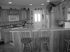
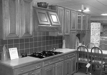
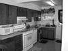
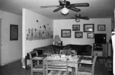
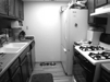
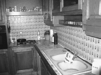
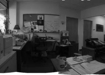
Kitchen	0.550					LivingRoom	InsideCity	Office	Bedroom
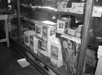
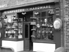
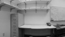
Store	0.490					InsideCity	Kitchen	LivingRoom	InsideCity
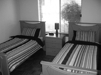
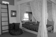
Bedroom	0.420		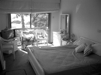			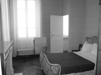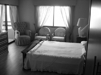LivingRoom	Kitchen	Office	LivingRoom
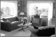
LivingRoom	0.470					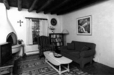Bedroom	Bedroom	Bedroom	Bedroom
Office	0.890					Bedroom	InsideCity	Kitchen	LivingRoom
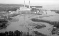
Industrial	0.520					TallBuilding	TallBuilding	Highway	Kitchen
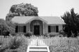
Suburb	0.940					Street	OpenCountry	Coast	TallBuilding
InsideCity	0.640					Street	Kitchen	Store	Street
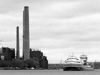
TallBuilding	0.790					Suburb	OpenCountry	InsideCity	Forest
Street	0.760					LivingRoom	InsideCity	LivingRoom	OpenCountry
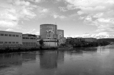
Highway	0.800					Store	Coast	OpenCountry	Coast
OpenCountry	0.460					Forest	Industrial	Coast	Coast
Coast	0.770					Highway	OpenCountry	OpenCountry	Mountain
Mountain	0.790					OpenCountry	Coast	OpenCountry	LivingRoom
Forest	0.930					Mountain	Mountain	OpenCountry	Mountain
Category name	Accuracy	Sample training images		Sample true positives		False positives with true label		False negatives with wrong predicted label

Submitted Results

This section details the parameters and results for the submitted code that is meant to run in less than 10 minutes for each pipeline. I tried to make sure that the code ran as fast as possible, while still being just over the minimum requirement. I found that some other parameters should run in time and produce even better accuracy, but I wanted this to run quickly for grading purposes. I want to note that for the Bag of Words model, changing the SIFT_step to 8 should still run in well under 10 minutes while producing higher accuracy well within range.

The vocabulary that is submitted with the assignment has a vocab_size of 200 and a SIFT step size of 10

Tiny Images + KNN

For Tiny Images and the K-Nearest Neighbor classifier, the submitted code should produce 20.7% accuracy. The relevant parameters for this are a tiny image size of 16x16, as well as a K value of 5 for the KNN classifier

Bag of Words + KNN

For Bag of Words and the K-Nearest Neighbor classifier, the submitted code should produce 48.9% accuracy. The relevant parameters for this are a step size of 10 for the bag of words model, as well as a K value of 5 for the KNN classifier

Bag of Words + SVM

For Bag of Words and the Linear SVM classifier, the submitted code should produce about 59.4% accuracy. The relevant parameters for this are a step size of 10 for the bag of words model, as well as a lambda value of .0001 for the linear SVM

Best Results for 3 Pipelines

Pipeline	Accuracy
Tiny Images (16x16) + KNN (K = 5)	~20.7%
Bag of Words (10 step) + KNN (K = 5)	~48.9%
Bag of Words (10 step) + SVM (L = .0001)	~59.4%

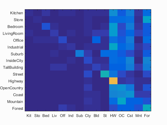
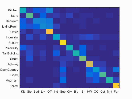
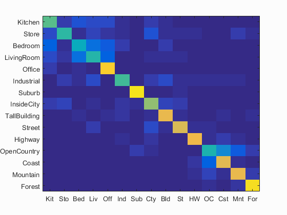
Confusion Matrices

All best results were obtained with a vocabulary size of 200, using a step of 10 for the vl_dsift