Raj Prateek Kosaraju

Representation

Tiny images representation

The "tiny image" representation (inspired by the work of Torralba, Fergus, and Freeman) is the simplest possible image representation. We simply resizes each image to 16*16 and make sure the images have zero mean and unit length (normalize them).

The matlab code to do the same is provided below:

image_feats = zeros(size(image_paths,1),16*16);

for imageIndex = 1:size(image_paths,1)
    current_image = imread(char(image_paths(imageIndex)));
    new_image = imresize(current_image, [16 16]);
    new_image_single_row = reshape(new_image, [1 16*16]);
    new_image_single_row = double(new_image_single_row);
    new_image_single_row = new_image_single_row - mean(new_image_single_row);
    new_image_single_row = new_image_single_row./norm(new_image_single_row);
    image_feats(imageIndex,:) = new_image_single_row;
end

Bag of SIFT representation

Building the Vocabulary

we first need to establish a vocabulary of visual words. We form this vocabulary by sampling SIFT features from our training set and then clustering them with kmeans. The number of clusters would be equal to the vocubulary size that we chose. To classify new SIFT feature we observe, we can figure out which class it belongs to as long as we save the centroids of our original clusters. These centroids are our visual word vocabulary. The code illustrates how we can build the vocabular in matlab

num_images = size(image_paths,1);

sampled_sift = zeros(128,1);
counter = 1;
for image_index = 1:num_images
    cur_image = imread(char(image_paths(image_index)));
    cur_image_single = im2single(cur_image);
    [locs, sift_feats] = vl_dsift(cur_image_single, 'Step', 15, 'Fast');
    num_curr_feats = size(sift_feats,2);
    sampled_sift(:,counter:counter+num_curr_feats) = sift_feats(:,:);
    counter = counter + num_curr_feats;
end
size(samples_sift)
[centers, assignments] = vl_kmeans(sampled_sift, vocab_size);

vocab = single(centers');

Getting the bags

For each image, we sample SIFT descriptors and count how many SIFT descriptors fall into each cluster in our visual vocabulary. We do this by finding the nearest neighbor kmeans centroid for every SIFT feature. The following matlab code illustrates this very easily:

vocab_size = size(vocab, 1);

num_images = size(image_paths,1);
image_feats = zeros(num_images, vocab_size);
num_dists_to_consider = 15;

for image_index = 1:num_images
    histogram = zeros(vocab_size,1);
    z = image_index;
    cur_image = imread(char(image_paths(image_index)));
    cur_image_single = im2single(cur_image);
    [locs, sift_feats] = vl_dsift(cur_image_single, 'Step', 15, 'Fast');
    all_dist = (vl_alldist2(uint8(vocab'),uint8(sift_feats)));
    [Y, sortedIndices] = sort(all_dist,1);
    for j = 1:num_dists_to_consider
       for feature_i  = 1:size(all_dist,2)
           vocab_to_vote = sortedIndices(j,feature_i);
           histogram(vocab_to_vote)  = histogram(vocab_to_vote)+1;
       end
    end    
    %normalize and store
    image_feats(image_index, :) = (histogram/norm(histogram))';  
end
end

Classification

K Nearest Neighbors

This is a very popular classification technique. When tasked with classifying a test sample into a particular category, we simply find the "nearest" K training examples and assign the test case the label of the most frequently occuring class. We can also implement more advanced strategies where we weigh each class depending on how "far" the training example was, from our test sample.

Linear SVM

The next classifier is built by training multiple 1-vs-all class linear SVMS to operate in the bag of SIFT feature space. Linear classifiers are one of the simplest learning models. The feature space is partitioned by a learned hyperplane and test cases are categorized based on which side of that hyperplane they fall on. We simply query each model for each test example and check which one is the most confident about its prediction. That model will determine the class for that example. The matlab code illustrates the same:

categories = unique(train_labels); 
num_categories = length(categories);
num_training = size(train_image_feats, 1);
num_test = size(test_image_feats,1);
num_each_test = size(test_image_feats,2);
train_weights = zeros(num_categories, num_each_test);
train_offsets = zeros(num_categories, 1);

for category_index = 1 : num_categories
    curr_labels = zeros(num_training,1);
    curr_labels = curr_labels -1;
    curr_labels(strcmp(char(categories(category_index)), train_labels)) = 1;
    [W, B] = vl_svmtrain(train_image_feats', curr_labels,  0.0001);
    train_weights(category_index,:) = W';
    train_offsets(category_index) = B;
end
predicted_categories = cell(num_test,1);
for test_image = 1:num_test
    maxScore = intmin('int8') ;
    bestCategory = '';
    for category_index = 1 : num_categories
        cur_score = train_weights(category_index,:)*(test_image_feats(test_image,:)') + train_offsets(category_index);
        if cur_score > maxScore
            maxScore = cur_score;
            bestCategory = char(categories(category_index));
        end
    end
    predicted_categories{test_image} = bestCategory;
end
end

Results

Tiny Images representation and KNN

I resized images to 16*16 and set the K to 10. I also normalized the images and made them zero mean. Normalization improved the accuracy by around 3%. Extra credit results are discussed later.

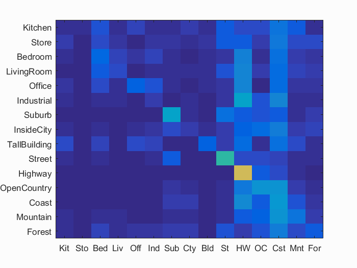
Accuracy (mean of diagonal of confusion matrix) is 0.213

Bag of SIFT representation and KNN

I used K = 10 here as well. I set the step to 15 and used the Fast parameter while determining the SIFT features. I also normalized the histograms before storing them as features. These results are without any of the extra credit modifications.

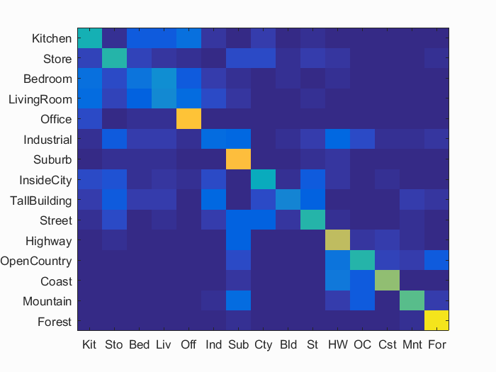
Accuracy (mean of diagonal of confusion matrix) is 0.514

Bag of SIFT representation and Linear SVM - Overall Best

Everything said earlier above bag of SIFT features still holds here. For the Linear SVM, I set the lambda to 0.0001 and trained a classifier for each class. This particular pipeline's results also includes the extra credit that is described in more detail at the end of the document.

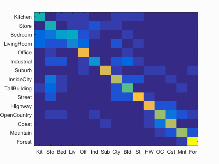
Accuracy (mean of diagonal of confusion matrix) is 0.620

Category name	Accuracy	Sample training images		Sample true positives		False positives with true label		False negatives with wrong predicted label
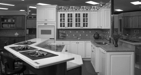
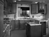
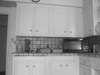
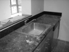
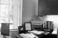
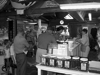
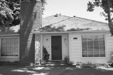
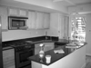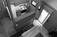
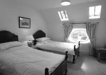
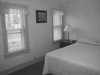
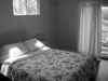
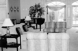
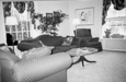
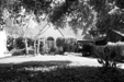
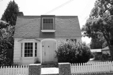
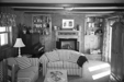
Kitchen	0.310					Bedroom	Store	Mountain	Bedroom
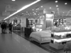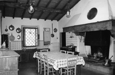
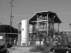
Store	0.260					Industrial	InsideCity	TallBuilding	Highway
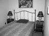
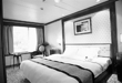
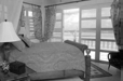
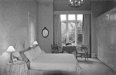
Bedroom	0.430		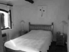			Office	InsideCity	Office	Kitchen
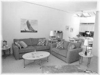
LivingRoom	0.080		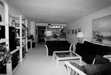			Kitchen	Bedroom	Industrial	Office
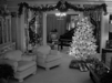
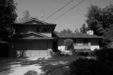
Office	0.970					Bedroom	InsideCity	Bedroom	Street
Industrial	0.240					LivingRoom	LivingRoom	InsideCity	Mountain
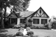
Suburb	0.950		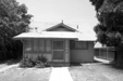			Store	Mountain	Street	InsideCity
InsideCity	0.510					LivingRoom	TallBuilding	Industrial	Suburb
TallBuilding	0.700					Bedroom	Industrial	Bedroom	InsideCity
Street	0.600					Suburb	LivingRoom	LivingRoom	Suburb
Highway	0.720					OpenCountry	OpenCountry	Suburb	Mountain
OpenCountry	0.500					Mountain	Coast	Forest	Mountain
Coast	0.810					OpenCountry	OpenCountry	OpenCountry	OpenCountry
Mountain	0.770					Store	Highway	Suburb	Suburb
Forest	0.910					OpenCountry	Mountain	Mountain	Mountain
Category name	Accuracy	Sample training images		Sample true positives		False positives with true label		False negatives with wrong predicted label

Above & Beyond

I tried to improve upon my best results above by trying these following approaches. I ran each of these independent of each other as I wanted to compare the improvements.

Soft assignment for visual words

I modified my code so that it considers the distance to the centroid while building the histogram. Hence, each feature adds some weight proportional to how far it is from each centroid.

           distance_of_vote = all_dist(j,feature_i)+1;
           actual_score = min(0,1/distance_of_vote);
           histogram(vocab_to_vote)  = histogram(vocab_to_vote)+actual_score;  
 

This modestly increased the accuracy by 2% over the existing result, to 23%.

Use cross-validation

I added the code required for performing a 10-fold cross-validation on the whole pipeline. It prints the mean accuracy in the end. Cross validation gives better results at times because of the change in the train and test sets between folds. The results for the first two folds for KNN and Tiny features were: 24.7% and 26%.

Experiment with many different vocabulary sizes

The initially reported results were for a vocab size of 200. Changing the vocab size to 50 resulted in 2% increase in accracy, 60.6%. Using a vocab size of 100 results in 59.7% and a vocab size of 150 resulted in 60.8%. I also tried a vocab size of 250, which resulted in an accuracy of 61.2%. Overall, all of them seemed to achieved better results than the initial size.

Modify training process to tune learning parameters

For chosing a value of lambda in SVM, the code tried different values of lambda and picks the one with the highest training accuracy. It then uses this lambda to build the classifiers. It picked the value of 0.0001 in my tests.
I also tried a similar approach for chosing the number of neighbors in KNN. It tries various values for K and choses the one that it finds the highest training accuracy for. It always picked 10 in my tests.

Improve the KNN classifier to be more competitive

I attempted to improve the KNN classifier by using an approach similar to soft assignment. Instead of just picking the most frequent class, I assigned scores to each class depending on the distance and picked the one with the highest score. This resulted in the tiny images + KNN pipeline performing slightly better, with an accuracy of 23.3%.