Project 4 - Scene Recognition with Bag of Words
This project focuses on using various types of features and classification techniques to attempting to classify scenes into one of 15 categories by training and testing on the 15 scene database. There are the combinations of features and classifiers that I have implemented.
- Tiny image features + Nearest Neighbor Classifier
- Bag of SIFT features + Nearest Neighbor Classifier
- Bag of SIFT features + Support Vector Machines
Tiny image features + Nearest Neighbor Classifier
It would be impossible to train and validate our classifiers on the whole image simply because of the size of required data. The tiny image mechanism shrinks the image to a very small size so that it can be used as a feature descriptor of the original image. This solution is not extremely desirable since most detail and high frequency cotent in the image is lost (it blurs the image) while shrinking it.
This part of the implementation was fairly straighforward. I made the images a size of 16 by 16 pixels. I made the design making the tiny images zero mean and unit length (normalizing them) to increase performance modestly because it becomes invariant to small changes.
The k-nearest neighbor classifier is based on the assumption that a feature is probably similar to another that is in close proximity to another in feature space.
I experimented with a different number of neighbors and with and without normalization. I implemented a weighted voting mechanism, which the first 'k' number of neighbors had a say in the classification of a sample. This was to minimize the impact of outliers. Accuracies after varying parameters is reported below.
Results
| Accuracy | K = 1 | K = 5 | K = 10 | K = 15 |
| Without Normalization | 0.202 | 0.191 | 0.190 | 0.197 |
| With Normalization | 0.225 | 0.215 | 0.213 | 0.221 |
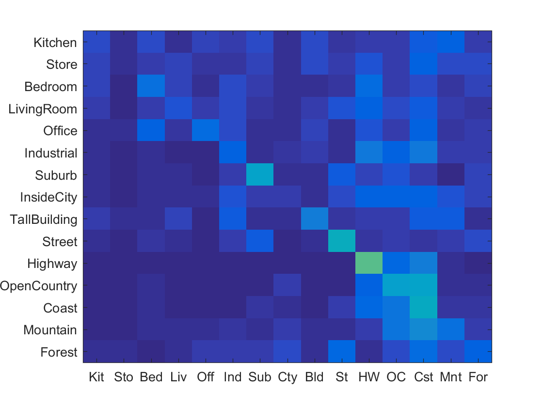
The best performing configuration seemed to be when k = 1 and with normalization. It happened that the neighbor voting did not increase accuracy. However, it could be due to the orientation of the feature space. The confusion matrix is as shown below.
Bag of SIFT features + Nearest Neighbor Classifier
The next pipeline used bag of words implementation that were derived from SIFT descriptors instead of shrunk training images. I used vl_dsift in order to obtain SIFT descriptors of each image. Then, I then compiled a descriptor that was formed from the bag of words by assigning each to a cluster using the nearest neighbor algorithm.
The design decisions I made were to vary vocabulary size from 50 to 400. I also varied step size.
I also performed the extra credit of using "soft assignment" to assign visual words to normalized histogram bins. I will report the difference in accuracy in this section for extra credit.
Note: I will be using k = 5 so that I can show the effects of soft assignment
Results
| Accuracy | Vocab size = 50, Step size = 10 | Vocab size = 100, Step size = 10 | Vocab size = 200, Step size = 10 | Vocab size = 400, Step size = 10 | Vocab size = 400, Step size = 20 | Vocab size = 400, Step size = 40 |
| With soft assignment | 0.406 | 0.448 | 0.503 | 0.503 | 0.473 | 0.438 |
| Without soft assignment | 0.389 | 0.428 | 0.481 | 0.481 | 0.461 | 0.402 |
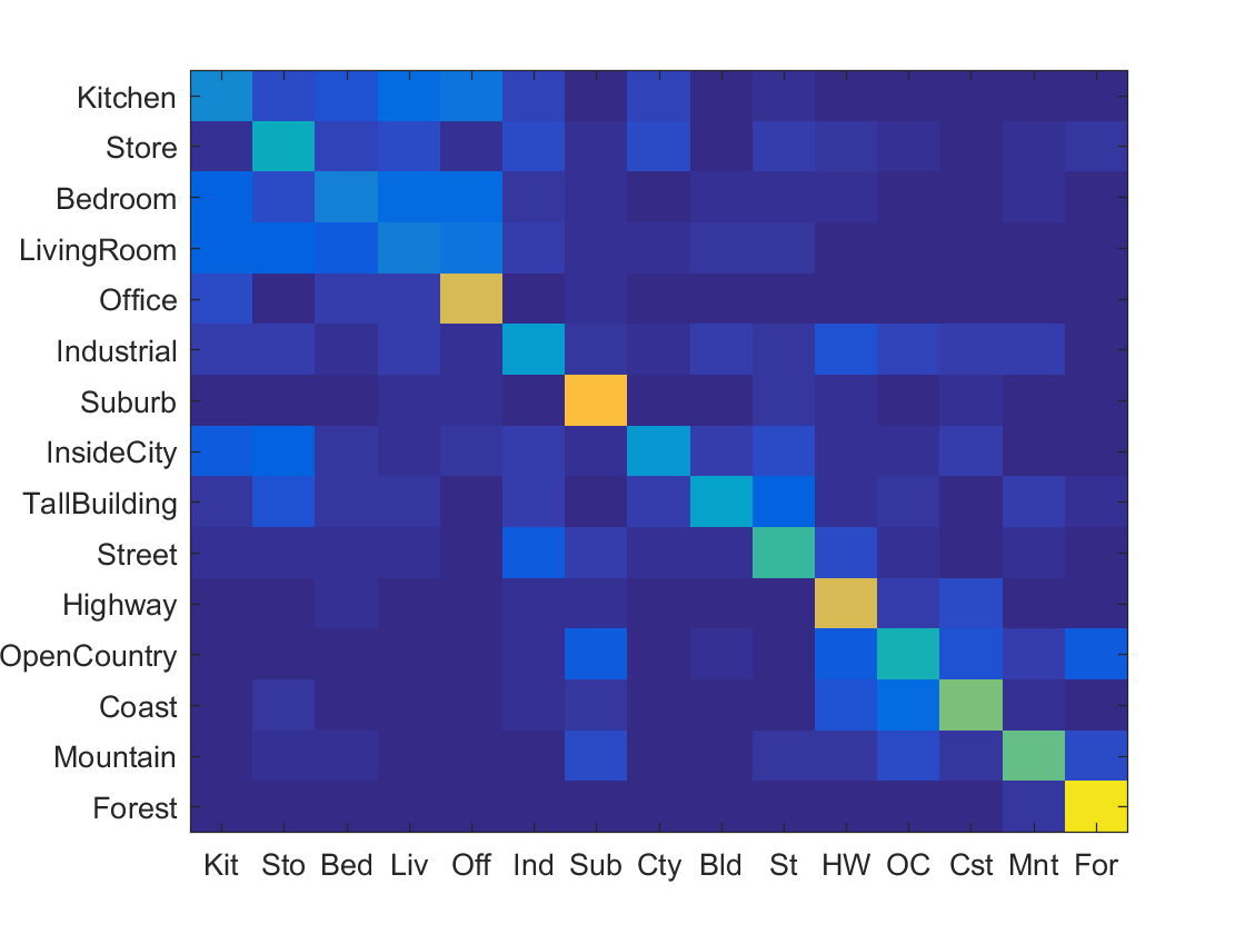
The best performing configuration seemed to be with soft assignment and with vocabulary size of 200 and step size of 10. The soft assignment did help accuracy as shown above, since it minimized the effect of outliers. The confusion matrix of the best configuration is as shown below.
Bag of SIFT features + Support Vector Machine Classifier
The next pipeline used bag of words implementation as before but used the Support Vector Machines classifier.
The linear SVM classifier tries to partition the feature space into one category or the other. I used the vl_svmtrain function from vlfeat's library. Every test feature was evaluated 15 SVMs and the most confident one is selected. Confidence is calculated as W*X + B where W and B are the learned hyperplane parameters from vlfeat's SVM function.
I experimented with different lambdas and vocabulary sizes.
Results
| Accuracy | Vocab size = 50 | Vocab size = 100 | Vocab size = 200 | Vocab size = 400 |
| Lambda = 0.00005 | 0.479 | 0.598 | 0.619 | 0.624 |
| Lambda = 0.0001 | 0.482 | 0.601 | 0.627 | 0.633 |
| Lambda = 0.0005 | 0.52 | 0.582 | 0.604 | 0.61 |
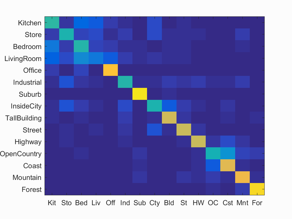
The best performing configuration seemed to be with vocabulary size of 400 and step size of 10 and lambda 0.0001. The confusion matrix of the best configuration is as shown below.

The accuracy (mean of diagonal of confusion matrix) was 0.633
Scene classification results visualization
Accuracy (mean of diagonal of confusion matrix) is 0.633
| Category name | Accuracy | Sample training images | Sample true positives | False positives with true label | False negatives with wrong predicted label | ||||
|---|---|---|---|---|---|---|---|---|---|
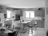
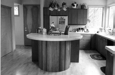
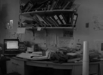
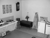
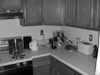
| Kitchen | 0.490 |  |
 |
 |
 |
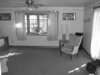 LivingRoom |
 Bedroom |
 InsideCity |
 InsideCity |
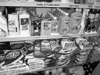
| Store | 0.460 | 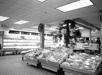 |
 |
 |
 |
 Street |
 OpenCountry |
 Kitchen |
 Bedroom |
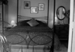
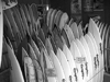
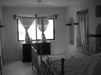
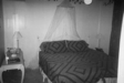
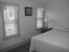
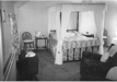
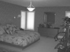
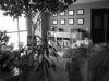
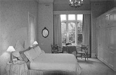
| Bedroom | 0.470 | 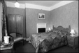 |
 |
 |
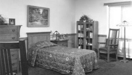 |
 Office |
 LivingRoom |
 Kitchen |
 Kitchen |
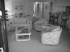
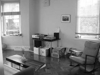
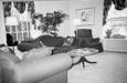
| LivingRoom | 0.210 | 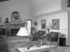 |
 |
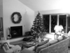 |
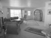 |
 Bedroom |
 Kitchen |
 Store |
 Bedroom |
| Office | 0.850 | 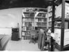 |
 |
 |
 |
 LivingRoom |
 Bedroom |
 LivingRoom |
 Kitchen |
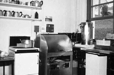
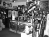
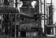
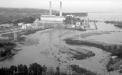
| Industrial | 0.480 | 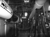 |
 |
 |
 |
 InsideCity |
 Kitchen |
 Store |
 Bedroom |
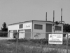
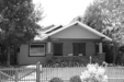
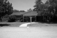
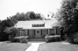
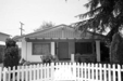
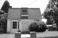
| Suburb | 0.940 | 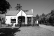 |
 |
 |
 |
 Industrial |
 LivingRoom |
 TallBuilding |
 TallBuilding |
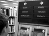
| InsideCity | 0.460 |  |
 |
 |
 |
 Street |
Kitchen |
 Bedroom |
 Store |
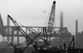
| TallBuilding | 0.740 |  |
 |
 |
 |
 InsideCity |
 InsideCity |
 Mountain |
 Industrial |
| Street | 0.730 |  |
 |
 |
 |
 Bedroom |
 Kitchen |
 TallBuilding |
 Highway |
| Highway | 0.730 |  |
 |
 |
 |
 OpenCountry |
 Industrial |
 Suburb |
 Street |
| OpenCountry | 0.440 |  |
 |
 |
 |
 Mountain |
 Forest |
 Coast |
 Mountain |
| Coast | 0.780 |  |
 |
 |
 |
 Store |
 OpenCountry |
 Suburb |
 OpenCountry |
| Mountain | 0.800 |  |
 |
 |
 |
 Forest |
 OpenCountry |
 Suburb |
 Street |
| Forest | 0.910 |  |
 |
 |
 |
 Mountain |
 TallBuilding |
 Mountain |
 Mountain |
| Category name | Accuracy | Sample training images | Sample true positives | False positives with true label | False negatives with wrong predicted label | ||||
Extra credit
The extra credit implemented is the following. It has already been shown in the previous sections, and explained as well as clearly reported with results with all the other design decisions in the previous sections.
- Experiment with many different vocabulary sizes and report performance - All pipelines
- Distance-based voting for KNN. The results were outlined in part 2