Project 4 / Scene Recognition with Bag of Words
The implementation consists of three major pipelines:
Tiny Images + Nearest Neighbors
In the function get_tiny_images, I read every image in the image_path. Then resize this image into a 16 x 16 image and then flatten this image. Thus for 1500 images I get a matrix of size 1500 x 256. I then subtract the mean from each point and divide the matrix by sum of aboslute values along each row, thus getting unit length and zero mean for each image.
In the Nearest Neighbors I use the vl_alldist2() to get the distance between the train and test features and then take the nearest neighbor for each image in the test set and get the corresponding label from the set of labels.
I get an accuracy of 21.8% with Tiny Images + Nearest Neighbors
Bag of SIFT + Nearest Neighbors
In build_vocabulary() function I use a step size of 4 for finding SIFT vectors. I use the 'fast' parameter while calculating the SIFT features. I then use kmeans to find the centers of the clusters and saved them as vocabulary which is vocab_size x 128 matrix. I am using a vocab size of 200 to create the vocabulary.
In the get_bag_of_sifts() function I use a step size of 6 for finding the SIFT vectors, along with the 'fast' parameter. I then divide the features into bins, where the number of bins is equal to vocab_size. In the end, I normalize the image_vectors and return this matrix.
I get an accuracy of 51.3% with Bag of SIFT + Nearest Neighbors
| Step Size in get_bag_of_sifts | Accuracy |
| 6 | 51.3% |
| 8 | 48.9% |
| 16 | 47.1% |
Note : The vocabulary size is 200 and step size in bag_of_sifts is 6
| Step Size in build_vocabulary | Accuracy |
| 4 | 51.3% |
| 8 | 49.7% |
| 16 | 45.6% |
Bag of SIFT + SVM
In the svm_classify function, I tried different values of lambda and the value 0.000005 gave me the best results. In this function I am using SVM for every category and then combining the results. Before finding SVM I am making the labels binary for each category, 1 implying that the image belongs to that category and -1 implies otherwise. Once I compute the W and B matrices for all categories I do a Wx + B and then find the indices with maximum confidence values. And then use these indices to get the predicted labels.
I get an accuracy of 64.3% with BAG of SIFT + SVM
Note : The vocabulary size is 200 and step size in bag_of_sifts is 6
| Lambda | Accuracy |
| 0.00005 | 60.0% |
| 0.00001 | 62.9% |
| 0.000005 | 64.3% |
Here is the summary of the accuracies I get after different implementations:
| Method | Accuracy |
| Tiny Images + Nearest Neighbors | 21.8% |
| Bag of SIFT + Nearest Neighbors | 51.3% |
| Bag of SIFT + SVM | 64.3% |
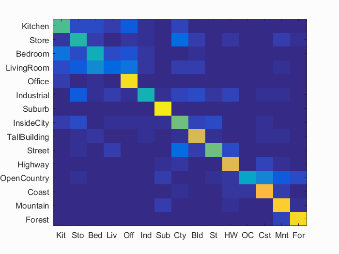
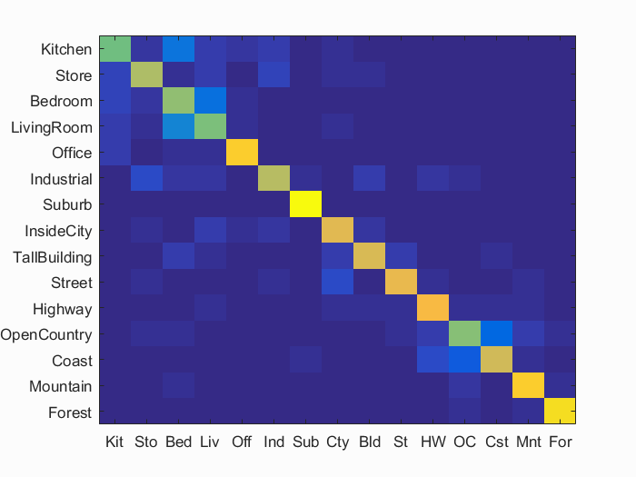
Accuracy (mean of diagonal of confusion matrix) is 0.643
| Category name | Accuracy | Sample training images | Sample true positives | False positives with true label | False negatives with wrong predicted label | ||||
|---|---|---|---|---|---|---|---|---|---|
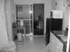
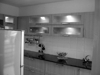
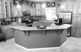
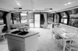
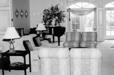
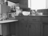
| Kitchen | 0.540 | 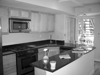 |
 |
 |
 |
 Bedroom |
 Store |
 Store |
 Office |
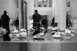
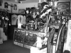
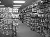
| Store | 0.480 | 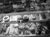 |
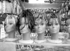 |
 |
 |
 LivingRoom |
 LivingRoom |
 Highway |
 Mountain |
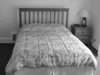
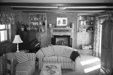
| Bedroom | 0.430 | 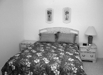 |
 |
 |
 |
 InsideCity |
 LivingRoom |
 Store |
Kitchen |
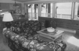
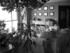
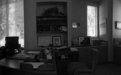
| LivingRoom | 0.150 |  |
 |
 |
 |
 InsideCity |
 Street |
 Store |
 TallBuilding |
| Office | 0.930 | 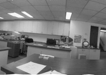 |
 |
 |
 |
 Store |
 InsideCity |
 Kitchen |
 Kitchen |
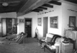
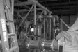
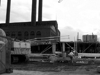
| Industrial | 0.440 | 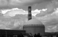 |
 |
 |
 |
 Store |
 TallBuilding |
 Highway |
 TallBuilding |
| Suburb | 0.960 |  |
 |
 |
 |
 OpenCountry |
 OpenCountry |
 Store |
 InsideCity |
| InsideCity | 0.590 |  |
 |
 |
 |
 Kitchen |
 Street |
 TallBuilding |
 Suburb |
| TallBuilding | 0.760 |  |
 |
 |
 |
 LivingRoom |
 Store |
 Mountain |
 Suburb |
| Street | 0.590 |  |
 |
 |
 |
 OpenCountry |
 InsideCity |
 TallBuilding |
 InsideCity |
| Highway | 0.780 |  |
 |
 |
 |
 OpenCountry |
Store |
 InsideCity |
 Industrial |
| OpenCountry | 0.380 |  |
 |
 |
 |
 Highway |
 Coast |
Suburb |
 Coast |
| Coast | 0.820 |  |
 |
 |
 |
 OpenCountry |
 OpenCountry |
 Mountain |
 Highway |
| Mountain | 0.880 |  |
 |
 |
 |
TallBuilding |
 TallBuilding |
 Forest |
 Forest |
| Forest | 0.920 |  |
 |
 |
 |
Mountain |
 OpenCountry |
 Street |
 Mountain |
| Category name | Accuracy | Sample training images | Sample true positives | False positives with true label | False negatives with wrong predicted label | ||||
Extra Credits
Gaussian Pyramid
I have included this file as gaussian_pyramid.m, in this function I use the impyramid function for two levels for each image to form the histogram.
I get an accuracy of 65.2% using the following settings:
Gist
The code is included in the file gist.m, in this file I am using vl_dsift function with a step size of 6 and Fast parameter, to compute the SIFT_features. I am then using LMgist function to get gist vectors and then randomly sampling 500 vectors from these and concatenating them to each image vector. Note: I am only normalizing the section of the vector obtained from SIFT vectors for every image.
I get an accuracy of 64.4% using the following settings:
Fisher
Fisher involves two steps: fisher_vocabulary(), in this function I use a stepSize of 4 and binsize of 16 to get SIFT features using the fast parameter. I then use the vl_gmm function to compute the means, covariances and posteriors from these SIFT features and save them as gmm_means, gmm_covariances and gmm_posteriors.
The fisher_vocabulary() function will only run when the above mentioned matrices are not there in the memory. Then these matrices are used in fisher.m file. In this file I basically use a stepSize of 2 to compute the SIFT features and then using vl_fisher I compute the fisher vector for each image. The size of this vector is vocab size (200) times 128 times 2.
I get an accuracy of 75.9% using the following settings:
Visualization for Fisher implementation:
Accuracy (mean of diagonal of confusion matrix) is 0.759
| Category name | Accuracy | Sample training images | Sample true positives | False positives with true label | False negatives with wrong predicted label | ||||
|---|---|---|---|---|---|---|---|---|---|
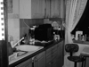
| Kitchen | 0.590 |  |
 |
 |
 |
 Store |
 Office |
 Bedroom |
 Store |
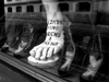
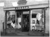
| Store | 0.680 |  |
 |
 |
 |
 InsideCity |
 Industrial |
 LivingRoom |
 TallBuilding |
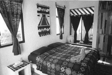
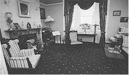
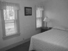
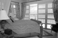
| Bedroom | 0.640 |  |
 |
 |
 |
 Mountain |
 LivingRoom |
 LivingRoom |
 LivingRoom |
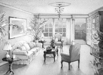
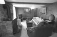
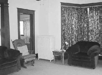
| LivingRoom | 0.600 |  |
 |
 |
 |
 Store |
 TallBuilding |
 Kitchen |
 Bedroom |
| Office | 0.890 |  |
 |
 |
 |
 Kitchen |
 Bedroom |
 Kitchen |
 LivingRoom |
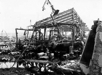
| Industrial | 0.690 | 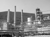 |
 |
 |
 |
 Kitchen |
 Bedroom |
 Suburb |
 Bedroom |
| Suburb | 0.990 |  |
 |
 |
 |
 LivingRoom |
 Coast |
 InsideCity |
|
| InsideCity | 0.780 |  |
 |
 |
 |
 Street |
 Street |
 Office |
 Street |
| TallBuilding | 0.760 |  |
 |
 |
 |
 Store |
 Bedroom |
 Street |
 InsideCity |
| Street | 0.790 |  |
 |
 |
 |
 TallBuilding |
 OpenCountry |
 Kitchen |
InsideCity |
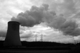
| Highway | 0.820 |  |
 |
 |
 |
 Industrial |
 OpenCountry |
 Coast |
 Mountain |
| OpenCountry | 0.610 |  |
 |
 |
 |
 Coast |
 TallBuilding |
 Coast |
 Bedroom |
| Coast | 0.740 |  |
 |
 |
 |
 OpenCountry |
 OpenCountry |
 Highway |
 OpenCountry |
| Mountain | 0.880 |  |
 |
 |
 |
Highway |
 Street |
 Suburb |
 OpenCountry |
| Forest | 0.930 |  |
 |
 |
 |
 Mountain |
 OpenCountry |
 OpenCountry |
 OpenCountry |
| Category name | Accuracy | Sample training images | Sample true positives | False positives with true label | False negatives with wrong predicted label | ||||
Spatial Pyramid
In the spatial_pyramid.m file I am computing 21 histograms instead of a single histogram in bag of sifts. The first histogram is computed using the entire image. Then I divide the image into 4 quadrants and compute a histogram based on the location of each SIFT vector. Then I divide the image into 16 quadrants and again compute 16 histograms based on the location of SIFT vectors. Then after normalizing these histograms separately for each step, I append them to form one image vector.
Thus this results in a number_of_images x (vocab_size * 21) size vector.
I get an accuracy of using the following settings:
The algorithm takes too long to run for stepSize 4, though it does give a slightly better accuracy.
Cross Validation
I have implemented cross validation in the proj4_cross_validation.m file. For each iteration I subsample 100 images for each category from the chosen images. I subsample it with replacement. And then call the bag_of_sifts with SVM classifier.
Here is the summary of the cross validation implementation:
| Iterations | Average Accuracy | Standard Deviation |
| 1 | 64.10% | 0.00% |
| 2 | 62.47% | 2.07% |
| 5 | 62.98% | 3.67% |
| 10 | 63.87% | 2.91% |
Different Vocabulary Sizes
Here is the summary of the accuracies I obtain by changing vocab_sizes and keeping the rest of the SIFT paramters same (similar to bag_of_sift + SVM implementation):
| Vocab_Size | Accuracy |
| 10 | 60.9% |
| 20 | 60.2% |
| 50 | 61.8% |
| 100 | 63.6% |
| 200 | 64.3% |
| 400 | 64.8% |
| 1000 | 63.9% |