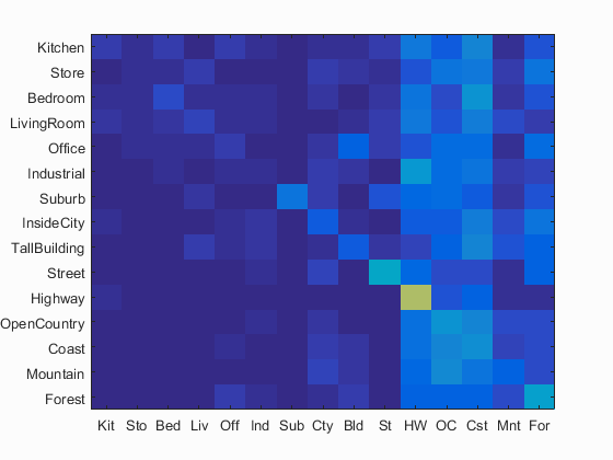
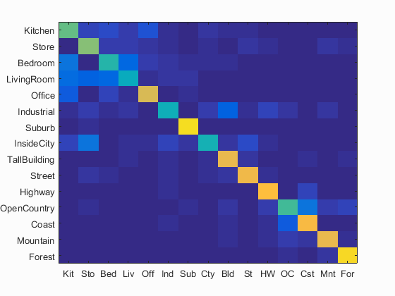
Confusion Matrix for Tiny Images and Nearest Neighbor Classifier. 19.1% Accuracy
The goal of this project was to train a model to recognize the scene of each image in the test set after being trained on the training set. To achieve this goal, a series of better learners and representations were created. Specifically tiny image and bag of SIFT words were independently used as features for scene detection, and nearest neighbor and support vector machines were tested as classifiers.
The simplest feature used was Tiny Images. For this feature, the input images were read in, then resized to a 16x16 pixel square. Overall this serves as a poor feature and was mostly used here as a baseline for comparison with SIFT features. An equally simple classifier is the Nearest Neighbor classifier. This one simply matches each test image by comparing it with the closest training image and chosing its class. With the Tiny Images feature, this usually meant the image that had a similar level of brightness as that and some other low frequency elements of the image are most of what was conveyed by the tiny image features. Overall, this combination managed to score an accuracy level of only 0.191.
Confusion Matrix for Tiny Images and Nearest Neighbor Classifier. 19.1% Accuracy
After establishing a baseline with Tiny Images, it was time to create a proper feature representation. To create a bag of SIFT words, it was first important to establish the alphabet to be used. Essentially, rather than record every single possible SIFT feature that may appear in an image at our given step size, we instead establish a number of "central" SIFT features by calculating all SIFT features possible in our training set, then sort them into a fixed number of clusters, say 200, using K-means clustering. Because this step is time intensive, after the vocabulary matrix is computed, it is saved to disk and reloaded for future computations. For most of my experiments, I created my vocabulary out of SIFT features that were of size 8x8 and calculated every 8 steps for each image and clustered them into 200 clusters. When I later tuned for best performance, I kept most of these parameters intact here, except clustered to 300 points instead.
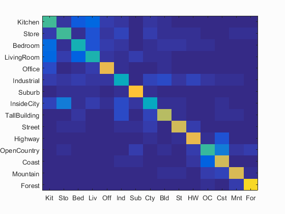
After the vocabulary was built, it could be used in order to engineer the features for each image. To do this, SIFT features were calculated for each image. Then every SIFT feature was sorted into its nearest cluster. Finally the clusters were binned to create a histogram recording the frequency of each cluster within the image. For these steps, again a step size of 8 and a SIFT size of 8x8 were used as they gave me the best results. As for those results, when paired with Nearest Neighbor classification, an accuracy score of 0.511 was achieved. Over a 250% improvement over Tiny Images.
Confusion Matrix for Bag of SIFT Words and Nearest Neighbor Classifier. 51.1% Accuracy
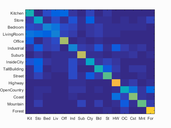
Finally, the Support Vector Machine classifier was used. Linear SVMs seek to find the linear divider with the biggest margin between the two classes of points. This is beneficial as it allows the model to trust the data as little as possible and in return tends to get good results even when the number of features are much higher the size of the data set (assuming the data is nearly linearly separable). Linear SVMs also tend to be much lower variance than 1 Nearest Neighbor which means that it is less prone to noise within the data set and will try to find more general patterns rather than just always looking up the closest example. As mentioned earlier, though, SVMs create a line that best separates, two classes of data. In order to tackle the multi-class problem here, it was necessary to train the SVMs in a One-vs-All manner where each class is checked individually and then the most confident class is selected. When the data is not completely linearly separable then some miss-classifications must be allowed. How much these miss-classifications in the training set are allowed to influence the generation of the hyperplane is dependent on the regularization parameter, lambda. In my experiments, a lambda parameter of 0.0001 got the best performance. With SIFT words as described earlier and the linear SVM, an accuracy score of 0.636 was achieved.
Confusion Matrix for Bag of SIFT Words and Linear SVM Classifier. 63.6% Accuracy
Out of curiosity, I decided to test out how well SVMs work with Tiny Image features rather than sift. Seeing as how SVMs worked so well with SIFT words I figured that they would still perform alright on the simpler feature, albeit not as well. In reality, this combination was by far the worst performing. Total accuracy for this combination was 0.113, however that only tells half the story. In the confusion matrix below, you can see that there is no discernable diagonal line of accurate predictions at all. Rather, most objects seem to have been classified as either a Bedroom, LivingRoom, or Mountain. These very poor results seem to indicate that the features were highly nonlinearly separable and as such the SVM was unable to create a good divider for the different classes. Tiny images puts a lot of emphasis on lighting and position of objects in an image, of which a lot of these features are irrelevant to the classifier and bag of SIFT words naturally filters out.
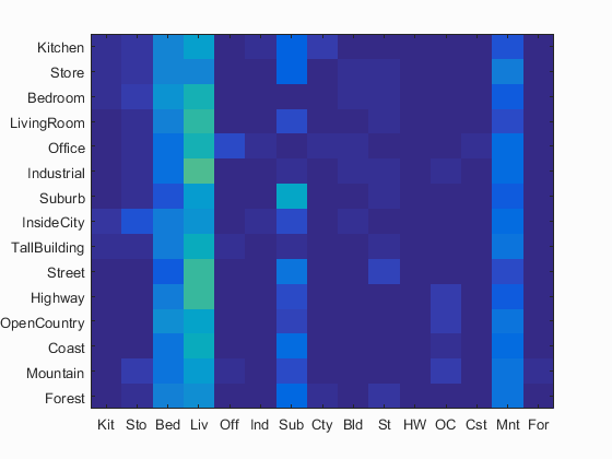
Confusion Matrix for Tiny Images and Linear SVM Classifier. 11.3% Accuracy
In order to really see how well I could push SVMs and Bag of SIFT words, I decided to mess with parameters further to improve performance. While changing most parameters did not have much effect, increasing the vocabulary size brought about a noticable improvement to accuracy in exchange for higher computation time to generate the vocabulary in the first place. This improved accuracy score was a 0.673 or 67.3%. Below I have included once again the confusion matrix for this pairing as well as an example of the images that the classifier trained on, succeeded on, and failed to classify both positively and negatively. What these reveal is that interiors such as Bed and Living Rooms tend to perform poorly while more outdoors scenes such as suburbs, coasts, and highways have the highest accuracies.
Confusion Matrix for Bag of SIFT Words with a vocab size of 300 and Linear SVM Classifier. 67.3% Accuracy
| Category name | Accuracy | Sample training images | Sample true positives | False positives with true label | False negatives with wrong predicted label | ||||
|---|---|---|---|---|---|---|---|---|---|
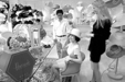
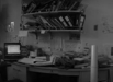
| Kitchen | 0.570 |  |
 |
 |
 |
 Bedroom |
 LivingRoom |
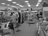
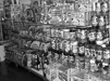
 Store |
 Office |
| Store | 0.620 | 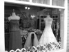 |
 |
 |
 |
Kitchen |
 LivingRoom |
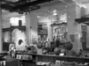 LivingRoom |
 LivingRoom |
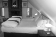
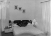
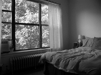
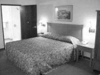
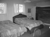
| Bedroom | 0.470 |  |
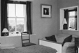 |
 |
 |
 Store |
 LivingRoom |
 Suburb |
 Industrial |
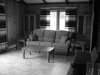
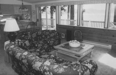
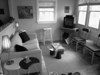
| LivingRoom | 0.410 | 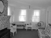 |
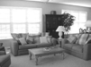 |
 |
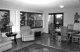 |
 Bedroom |
 Bedroom |
 Bedroom |
 Store |
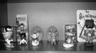
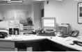
| Office | 0.750 |  |
 |
 |
 |
 InsideCity |
 Bedroom |
 Kitchen |
 Suburb |
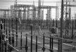
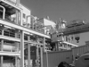
| Industrial | 0.430 | 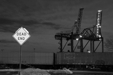 |
 |
 |
 |
 Coast |
 LivingRoom |
 TallBuilding |
 TallBuilding |
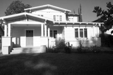
| Suburb | 0.930 |  |
 |
 |
 |
 Industrial |
 OpenCountry |
 Office |
 LivingRoom |
| InsideCity | 0.440 |  |
 |
 |
 |
 LivingRoom |
 Bedroom |
 Suburb |
 Store |
| TallBuilding | 0.790 |  |
 |
 |
 |
 Industrial |
 InsideCity |
 Street |
| Street | 0.800 |  |
 |
 |
 |
 Store |
 Industrial |
 Store |
 TallBuilding |
| Highway | 0.840 |  |
 |
 |
 |
 Suburb |
 Mountain |
 Industrial |
 Mountain |
| OpenCountry | 0.520 |  |
 |
 |
 |
 Mountain |
 Forest |
 Coast |
 Street |
| Coast | 0.820 |  |
 |
 |
 |
 Highway |
 OpenCountry |
 OpenCountry |
 OpenCountry |
| Mountain | 0.790 |  |
 |
 |
 |
 Industrial |
 Forest |
 Coast |
 OpenCountry |
| Forest | 0.910 |  |
 |
 |
 |
 Store |
 OpenCountry |
 Mountain |
 OpenCountry |
| Category name | Accuracy | Sample training images | Sample true positives | False positives with true label | False negatives with wrong predicted label | ||||