Project 4: Scene Recognition with Bag of Words
In this project we attempt to do scene recognition on various test images. We implement different feature extraction methods and different classifiying methods. For feature extraction tiny images and bag of SIFT features are implementd. For classification, we implement nearest neighbor and a 1 vs all linear SVM. The flow of this process is pretty simple: for all the images, training and test, we extract features, we then classify each test image based on some metric using the training images as reference.
Tiny Images
Tiny images is a simple and poor way to extract features. It simply resizes the image in to a 16x16 image. It then takes this matrix and converts it to a vector 256 elements long. This is now the 'feature' that represents this image. This is a very simple and over simplified feature extraction method, and therefore does not produce very accurate results.
Nearest Neighbor
Nearest neighbor is the simplest type of classifier. In this classifer, we find the distance from each test image to every train image. For every test image we find the closest training image and that is the label for the training image.
K-NN Extension
To implement K-NN each of the closest neighbors vote towards what the label should. The parameter k determines how many closest neighbors get a vote. The label with the highest vote amongst the k closest neighbors is assigned to the training label.
Bag of Sift
Build Vocabulary
In order to extract features using of bag of SIFT, we must first create a vocabulary of image "words" based on our training images and labels. To do this, we sample a certain number of SIFT features across all the training images. I decided to choose an equal number of features from every training image. For every image, I create a set of SIFT features, then randomly sample features from that set. Once I've gathered tens of thousands of SIFT features, I then create a vocabulary. I create a vocabulary through K-Means using VL's vl_kmeans function.
  % Read each image, get sift features, sample random set
  for i=1:size(image_paths,1)
    image = im2single(imread(image_paths{i}));
    [~, siftFeatures] = vl_dsift(image, 'step', siftStepSize);
    sampledSiftFeatures = [sampledSiftFeatures datasample(siftFeatures, siftFeaturesPerImage, 2)];
  end

  % Generate vocabulary
  [vocab, ~] = vl_kmeans(single(sampledSiftFeatures), vocab_size);
Feature Extraction
To extract features, we must describe each image with a bag of words using our pre-built vocabulary. For every image, we get it's SIFT features. We then find the distance of every extracted SIFT to every word in the vocabulary. The dimensions for a word and a SIFT feature are the same since we built the vocabulary using SIFT features. Then for each feature we select the closes word and that is the word for that SIFT feature. We create a histogram of all the words and this histogram becomes the feature descriptor for this image.
  % Generate SIFT features
  [~, siftFeatures] = vl_dsift(image, 'step', siftStepSize);

  % siftDistances(i,j) = local feature i distance to vocab word j
  siftDistances = vl_alldist2(single(siftFeatures), vocab);

  % Get words for each sift feature
  [~, indecies] = min(siftDistances, [], 2);

  % Create histogram of words based on local features
  siftHistogram = zeros(1, vocab_size);
  for j=1:size(indecies, 1)
    wordIndex = indecies(j, 1);
    siftHistogram(1, wordIndex) = siftHistogram(1, wordIndex) + 1;
  end
SVM Classifier
The final part was to create a linear Support Vector Machine (SVM) classifer. Since we have 15 different categories our method uses a 1-vs-all approach. For every category, we train an SVM and then evaluate each test image with it. At the end we have a distance matrix with a value for each test image evaluated by each SVM. For every image, the SVM that produced the most positive value is the category the test image corresponds to.
  % Find binary results with train labels, change 0s to -1s
  matchingIndices = double(strcmp(currentCategory, train_labels));
  matchingIndices(matchingIndices==0)=-1;

  % Get classifier for category
  [W B] = vl_svmtrain(train_image_feats', matchingIndices, LAMBDA);

  % Evaluate each test feature with this classifier
  distances(:,i) = W'*test_image_feats' + B;
Results (under 10 minutes)
| Feature | Classifier | Feature Params | Classify Params | Accuracy |
|---|---|---|---|---|
| Tiny Images | K-NN | 16x16 | k=10, L1 | 0.220 |
| Bag of Sift | K-NN | step size=8, fast enabled, vocab size=400, vocab samples=50,000, vocabstep size=1 | k=10, L1 | 0.515 |
| Bag of Sift | SVM | step size=8, fast enabled, vocab size=400, vocab samples=50,000, vocabstep size=1 | Lamda=0.001 | 0.630 |
Other Results
| Feature | Classifier | Feature Params | Classify Params | Accuracy |
|---|---|---|---|---|
| Bag of Sift | SVM | step size=5, vocab size=400, vocab samples=50,000, vocabstep size=1 | Lamda=0.00001 | 0.691 |
| Bag of Sift | SVM | step size=5, vocab size=10, vocab samples=50,000, vocabstep size=2 | Lamda=0.001 | 0.38867 |
| Bag of Sift | SVM | step size=5, vocab size=25, vocab samples=50,000, vocabstep size=2 | Lamda=0.001 | 0.52667 |
| Bag of Sift | SVM | step size=5, vocab size=50, vocab samples=50,000, vocabstep size=2 | Lamda=0.001 | 0.57867 |
| Bag of Sift | SVM | step size=5, vocab size=100, vocab samples=50,000, vocabstep size=2 | Lamda=0.001 | 0.58733 |
| Bag of Sift | SVM | step size=5, vocab size=250, vocab samples=50,000, vocabstep size=2 | Lamda=0.001 | 0.62133 |
| Bag of Sift | SVM | step size=5, vocab size=500, vocab samples=50,000, vocabstep size=2 | Lamda=0.001 | 0.65333 |
| Bag of Sift | SVM | step size=5, vocab size=1000, vocab samples=50,000, vocabstep size=2 | Lamda=0.001 | 0.64867 |
| Bag of Sift | SVM | step size=5, vocab size=2500, vocab samples=50,000, vocabstep size=2 | Lamda=0.001 | 0.65467 |
| Bag of Sift | SVM | step size=5, vocab size=5000, vocab samples=50,000, vocabstep size=2 | Lamda=0.001 | 0.64333 |
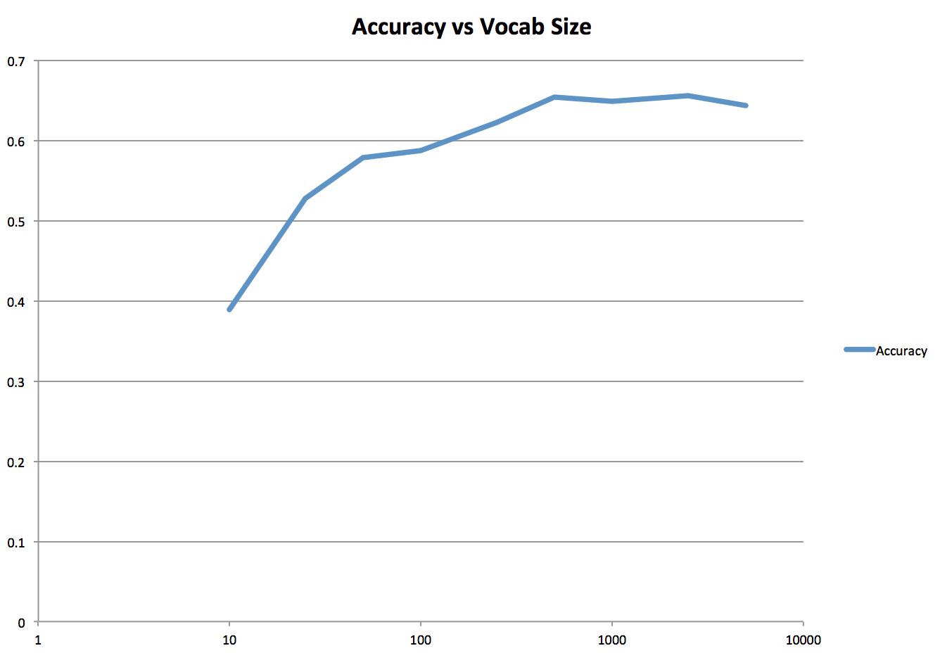
Variable Vocabulary Results
I also implmented a file named "multi_vocab.m" that creates vocabularies of varying sizes, and then runs bag of sift and SVM with those vocabularies. Vocabulary size increases the accuracy of classification, but soon levels off around 1000. A graph of the response is shown below, as well as a gif of all the confusion matrices generated.
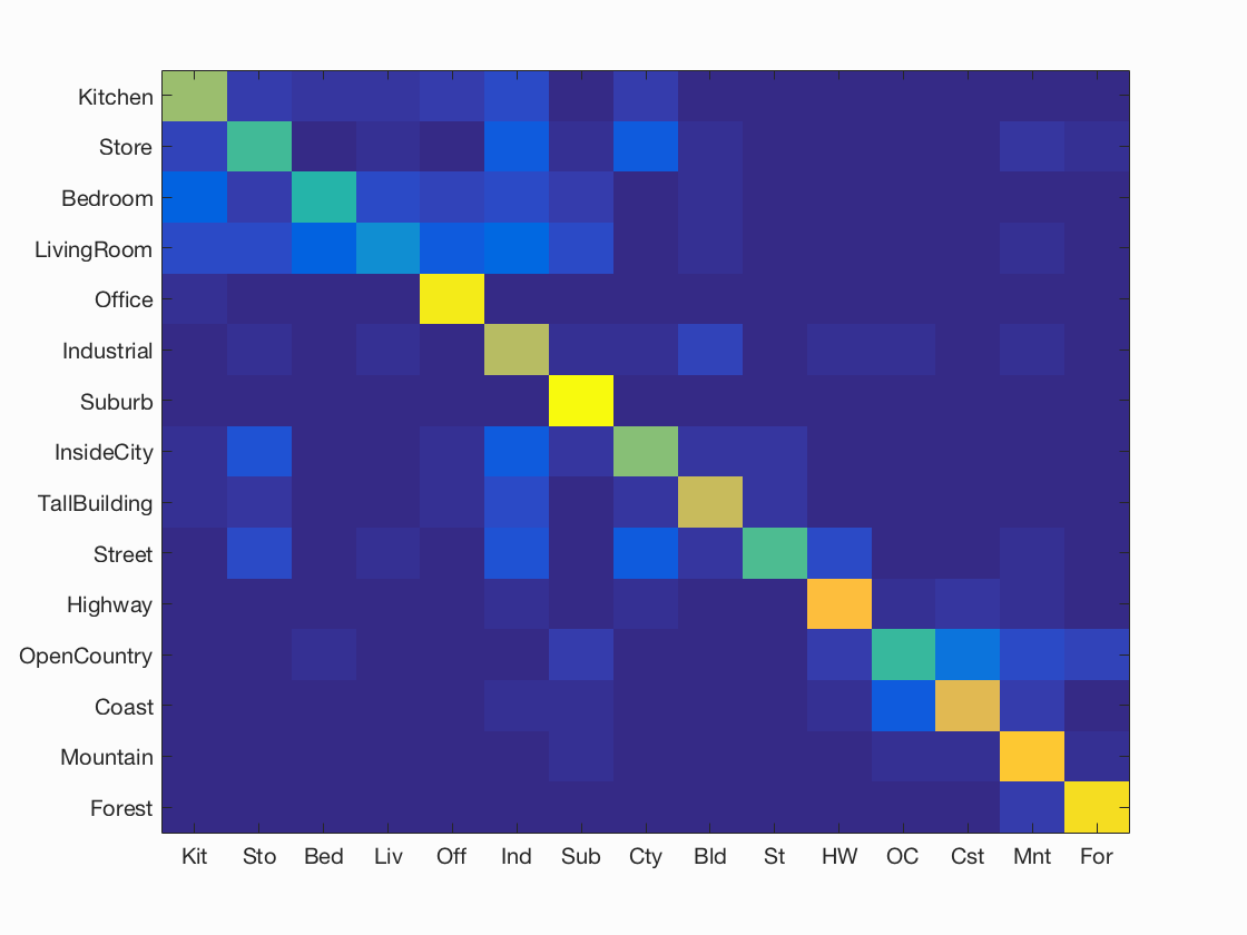
Confusion Matrices
Accuracy vs Vocab Size
Best Results
Accuracy (mean of diagonal of confusion matrix) is 0.691
| Category name | Accuracy | Sample training images | Sample true positives | False positives with true label | False negatives with wrong predicted label | ||||
|---|---|---|---|---|---|---|---|---|---|
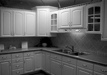
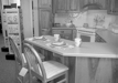
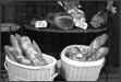
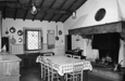
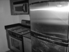
| Kitchen | 0.650 |  |
 |
 |
 |
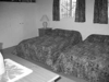
 Bedroom |
 Office |
 Store |
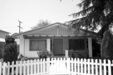
 Suburb |
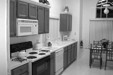
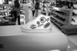
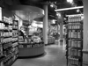
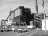
| Store | 0.530 |  |
 |
 |
 |
 Kitchen |
 Street |
 InsideCity |
 Industrial |
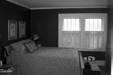
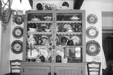
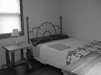
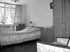
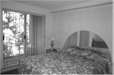
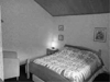
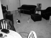
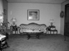
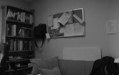
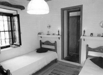
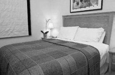
| Bedroom | 0.470 |  |
 |
 |
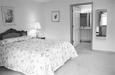 |
 LivingRoom |
 Store |
 LivingRoom |
 LivingRoom |
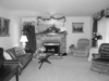
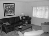
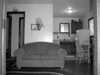
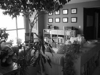
| LivingRoom | 0.290 |  |
 |
 |
 |
 Kitchen |
 Street |
 Bedroom |
 Office |
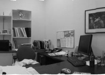
| Office | 0.960 | 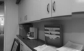 |
 |
 |
 |
 Bedroom |
LivingRoom |
 Bedroom |
Kitchen |
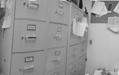
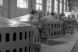
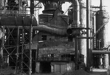
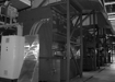
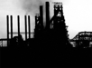
| Industrial | 0.690 | 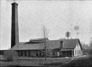 |
 |
 |
 |
 Bedroom |
 LivingRoom |
 TallBuilding |
 Highway |
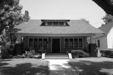
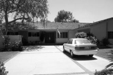
| Suburb | 1.000 | 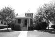 |
 |
 |
 |
 Mountain |
 Bedroom |
||
| InsideCity | 0.610 |  |
 |
 |
 |
 Highway |
 Street |
 Store |
 Industrial |
| TallBuilding | 0.720 |  |
 |
 |
 |
Industrial |
 InsideCity |
 InsideCity |
 Industrial |
| Street | 0.540 |  |
 |
 |
 |
 Highway |
 TallBuilding |
 InsideCity |
 TallBuilding |
| Highway | 0.830 |  |
 |
 |
 |
 Street |
 Coast |
 Suburb |
 Coast |
| OpenCountry | 0.510 |  |
 |
 |
 |
 Mountain |
 Mountain |
 Suburb |
 Forest |
| Coast | 0.770 |  |
 |
 |
 |
 OpenCountry |
 OpenCountry |
 OpenCountry |
 OpenCountry |
| Mountain | 0.860 |  |
 |
 |
 |
 Highway |
 OpenCountry |
 Coast |
 Forest |
| Forest | 0.930 |  |
 |
 |
 |
 OpenCountry |
 OpenCountry |
 Street |
 Mountain |
| Category name | Accuracy | Sample training images | Sample true positives | False positives with true label | False negatives with wrong predicted label | ||||