Project 4 / Scene Recognition with Bag of Words
In this project, we implement a classifier for scene recognition. The baseline for this task uses 2 methods to represent images and then 2 classification techniques. The 3 methods I will be comparing are:
- Baseline: Tiny image + nearest neighbor
- SIFT + nearest neighbor
- SIFT + SVM
Feature Representation
Tiny Image
This representation resizes an input image to a 16x16 size image and is an extremely simple way of representing an image. So while this isn't the best method for feature representation by any means, it'll work fine for our baseline metric.
Bag of SIFT
This method uses SIFT features to first create a vocabulary of visual words, which are clusters of features sampled from our training set. Lets say that the size of our vocabulary is v_size. For each new SIFT feature that we see from an image, we find which visual word that feature is closest to and then we have a histogram of v_size x 1, where each row is the count of how many SIFT descriptors from an image fall into each visual word cluster. The output of this is a histogram representation of the SIFT features classified into their respective visual words.
Classifiers
Nearest Neighbor
Given a test feature and a dataset of training features with labels, this classifier finds the training feature that is the "nearest" and assigns that label to the test feature. By "nearest", we mean closest in Euclidean (L2) distance in the feature space. While this is a simple classifier to implement, its downsides are in how easily outliers and training noise affect it. Here, I'm using 1st nearest neighbor, which is particularly easily affected by this; by using k nearest neighbors, with k larger than 1, errors due to this can be alleviated.
SVM
To use an SVM for multi-class categorization, I train it to be 1 vs all so that the output of the SVM is "in this class" or "not in this class". This method required that I train an SVM for each category. The classifier with the highest confidence was selected as the matched category.
Results
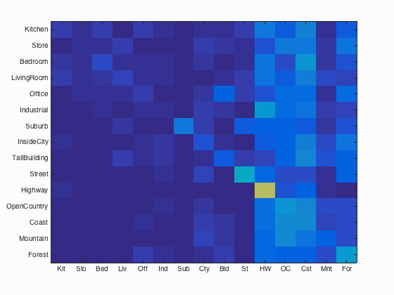
Baseline: Tiny image + nearest neighbor
Accuracy: 19.1%
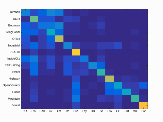
SIFT + nearest neighbor
Accuracy: 48.6%, a huge improvement from just using the tiny images as features.
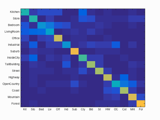
SIFT + SVM
Accuracy: 57.8%
Extra Credit
Validation Set
A validation set is commonly used to fine tune the parameters of a model. Given how long this program takes to run, I used a validation set of 500 images randomly chosen from the training set to see how my parameters were performing. Originally, I set the size of the validation set to 10% of the training set. This proved to be too small to show any trends in the way changing the parameters (the size of the vocabulary, in particular) affected the accuracy of the results. Changing the validation set to be larger helped, but the accuracy values of SIFT + 1-NN are high compared to what they were on the test set, with a 20% difference. I can only assume that this is due to overfitting; perhaps taking the validation set from the testing dataset or playing around with various sizes of the validation set would have been better.Experimental Design: Performance of varying parameters on a validation set
| Vocabulary Size | SIFT + NN | SIFT + SVM |
|---|---|---|
| 10 | 66.2 | 38.6 |
| 20 | 68.2 | 34 |
| 50 | 68.4 | 32.8 |
| 100 | 65.4 | 43.4 |
| 200 | 67.8 | 51.6 |
| 400 | 66.4 | 51 |
| Lambda (SVM) | .0000001 | .000001 | .00001 | .0001 | .001 | .01 |
|---|---|---|---|---|---|---|
| SIFT + SVM | 67.8 | 72.2 | 65 | 57.8 | 45 | 17 |
2-Fold Cross Validation
This method splits our dataset into two halves of equal size. We train on the first half and the test on the second, and then do the opposite (training on the second half, testing on the first). The benefit of this method of cross validation is that the training and test sizes are large and each data point ends up being part of both the training and testing dataset. Doing this results in 64.9% accuracy in one split and 65.9% accuracy in the other. The true error is estimated as the average error rate: 34.6%.K-Fold Cross Validation
Here, each train and test set are a random group of 100 images from the dataset and my K is 10. Here is the table for SIFT + NN:| K | 1 | 2 | 3 | 4 | 5 | 6 | 7 | 8 | 9 | 10 |
|---|---|---|---|---|---|---|---|---|---|---|
| Accuracy | 32 | 34 | 38 | 31 | 38 | 34 | 40 | 31 | 33 | 39 |
| K | 1 | 2 | 3 | 4 | 5 | 6 | 7 | 8 | 9 | 10 |
|---|---|---|---|---|---|---|---|---|---|---|
| Accuracy | 29 | 25 | 24 | 25 | 35 | 25 | 36 | 35 | 25 | 40 |
Kernel Codebook Encoding
This approach towards feature encoding weights visual words near the visual word assigned in the feature space, so that the influence of each feature is distributed across multiple visual words. I use k-nn to find the closest visual words to a feature and assign the weight to them based on the weighting equation. Applying this method significantly slowed down the code (which is why this section has been commented out--it'd push me past the 10 minute mark). It affected accuracy negatively when I set my k=4, decreasing the accuracy to 48.6%. At k=3, the accuracy is 44.5%. At k=5, the accuracy is 46.5%.Feature Representation: Adding Complementary Features
I added GIST descriptors to a new vocabulary file and modified my bags of SIFT code to work for the GIST descriptors. To make the SVM classifier take both descriptors into account, I concatenated the SIFT and GIST feature descriptors for each image and classified those descriptors (which required the vocab to be redone in this method as well). I thought about an alternate method of doing this, where I would run the SVM classifier separately on both bags of SIFT and bags of GIST. Then, to compute the final classification, I would compare the confidences of the SVM on the descriptors and see which class had the higher confidence frome either descriptor and that would be the predicted class. Additionally, I could experiment with weighting how much I value either the SIFT or GIST descriptor by changing the weights on the confidences when I'm comparing them to see which class I should select. With the first version, I ran out of time with this assignment, so I was still working on debugging the building vocabulary part.Fisher Vector Encoding
This uses vl_gmm to first create a Gaussian Mixture Model from the SIFT features of the training data. Then, for the training and testing data, I use vl_fisher to produce the encoding. The encoding is what's used instead of the feature vectors for classification. I couldn't figure out what the encodings actually represented though--they ended up being 100 (number of classes) x 400, but I couldn't figure out the classifier in the time remaining.