Sidney Durant

Project 4 / Scene Recognition with Bag of Words

This computer vision project involved classifying images based on various image features and classification methods. The image features in question were tiny images and bags of SIFT features. The classification methods in question were 1-nearest-neighbor and 1-vs-all-SVM. In this write up I will first describe the algorithms in question (and what decisions I made in regards to the parameters of these algorithms), and then I will show my results.

Feature 1: Tiny Images

This image feature is just a scaled version of the original image. The images are scaled to be 16x16 so that they can be made into a 1x256 feature vector. I decided not to crop the images before scaling the image because most of the images seem to have reasonable aspect ratios (so just turning them into square 16*16 images wouldn't be stretching them too much), and because I was worried about losing valuable information if I square cropped the images.

Feature 1: Bags of SIFT Features

This image feature is much more sophisticated than Tiny Images are. To further explain the Bags of SIFT features I should first explain how the visual vocabulary is built.

A visual vocabulary is a set of visual 'words'. Visual words are, in effect, image regions that are similar to each other. These similar image regions are found by getting SIFT features and then clustering them. For example, one visual word could be SIFT features that are similar to a black dot - dark in the center, and light on the outside. We find this visual vocab by finding SIFT features in all of the training images and then clustering them using k-means. The centroids of the regions generated by k-means are our visual words. I decided to make the vocabulary size quite large (400) because larger vocabularies are known to be more accurate (due to less 'discretization' error when 'rounding' features to their nearest visual word).

Bags of SIFT Features are simply histograms of the visual words for each category. We keep track of the frequency of each visual word in each category in the training set. In essence, we are finding what percentage of each visual word typically shows up in pictures of each category (e.g. what is the distribution of visual words in typical images of a forest). Later, when looking at the test set the classifiers try to find images with similar frequencies of visual words.

Classifier 1: Nearest Neighbor

K-Nearest-Neighbor classification algorithms in general find the K features that are nearest (to the feature in question) in the feature space, and take the mode of these K features to make a decision about what the feature in question is. What I implemented is 1-nearest-neighbor, which just finds the training image category whos features most closely resemble those of the image in question. The only parameter to modify here was K, and I stuck with 1 because I wanted to spend more time messing with SVM's than modifying KNN (because I knew that in the end, SVM would have the best results).

Feature 1: Linear Support Vector Machines

To make my explanation simpler, I'll assume that the features being used in this discussion of SVM's are tiny images. You can always replace tiny images with other features, however (and you'll see the results of doing this later). A support vector machine finds the hyperplane that best seperates 2 classes. SVM's are inherently binary classifiers, so we have to be clever in our application of them for this 15-category classification problem. To do this, we train 15 different linear-SVM's, and each linear SVM finds, for example, the confidence of a given image being a 'mountain' vs it being a 'non mountain'. To assign the class to the SVM, we pick the class that the SVM is most-confidently 'positive' about. There were several parameters to modify here, the crucial one being Lambda. I found that a Lambda = .0005 worked well on the given training/testing dataset.

Results:

Below I've shown the results for three different combinations of the above features & classifiers. Tiny Images with KNN was the worst performer. Tiny Images and SVM was in the middle, while Bag of Sifts + SVM had the best results. For all of these results, the parameters were as follows (which should be the same as what I submitted):

get_tiny_images:
• d = 16

nearest_neighbor:
• K = 1

build_vocabulary:
• Vocab size = 400
• SIFT size = 4
• step size = 10

get_bags_of_sifts:
• SIFT size = 4
• step size = 10

svm_classify:
• Lambda: 0.0005

Results for Tiny Images + KNN:

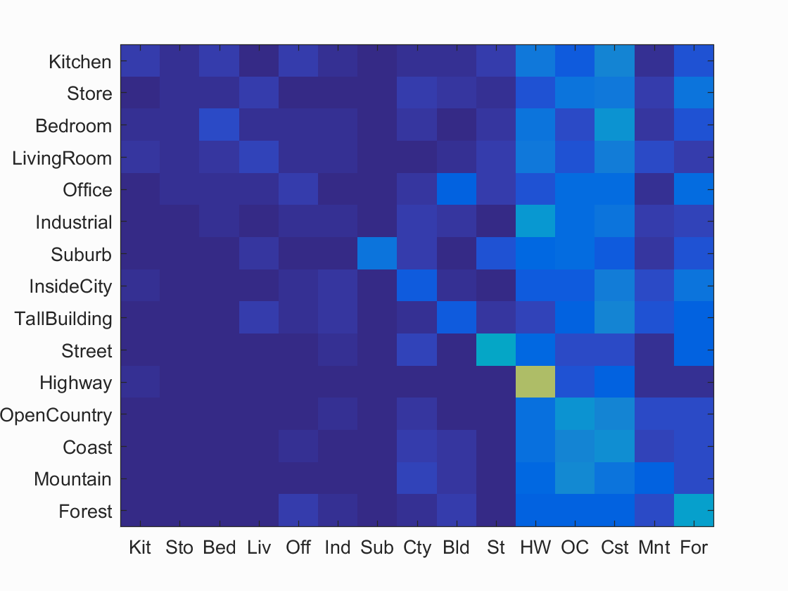
Accuracy (mean of diagonal of confusion matrix) is 0.191

Results for Bag of SIFTs + KNN:

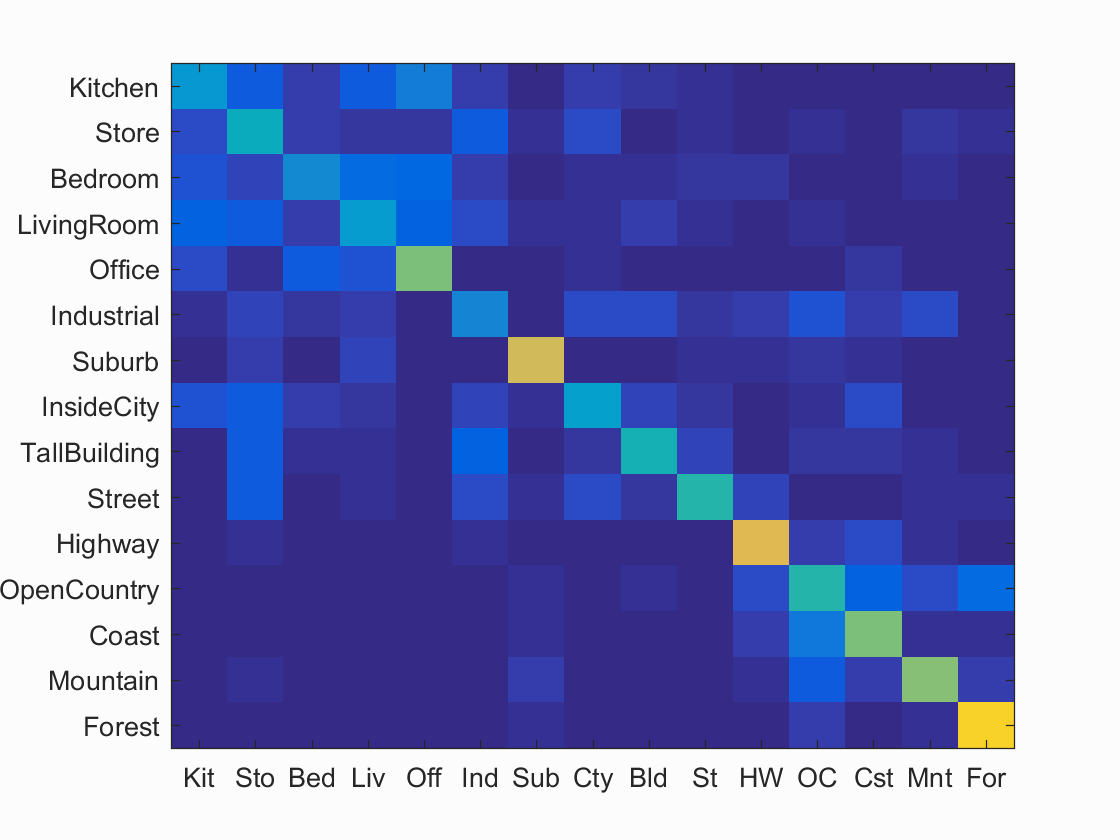
Accuracy (mean of diagonal of confusion matrix) is 0.507

Results for Bag of SIFTs + SVM:

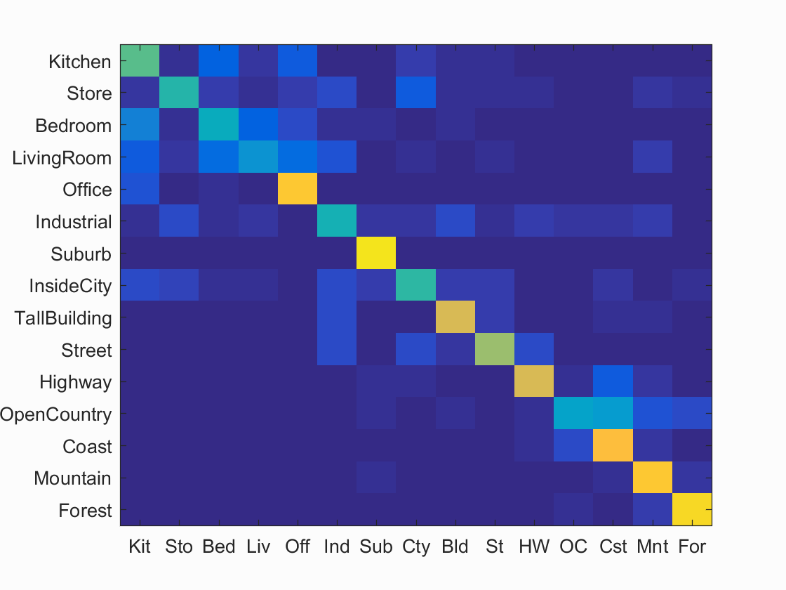
Accuracy (mean of diagonal of confusion matrix) is 0.642

Category name	Accuracy	Sample training images		Sample true positives		False positives with true label		False negatives with wrong predicted label
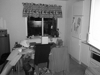
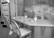
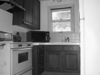
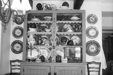
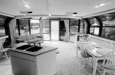
Kitchen	0.560					InsideCity	Store	Bedroom	Office
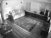
Store	0.480					Kitchen	LivingRoom	LivingRoom	InsideCity
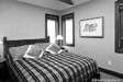
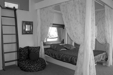
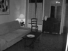
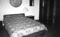
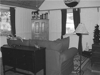
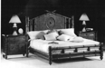
Bedroom	0.420		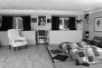			Kitchen	Store	Office	Kitchen
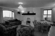
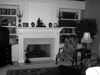
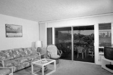
LivingRoom	0.300					Bedroom	Highway	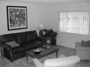TallBuilding	Mountain
Office	0.860		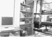			LivingRoom	Bedroom	Kitchen	Kitchen
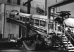
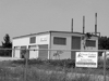
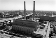
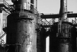
Industrial	0.440					LivingRoom	LivingRoom	Bedroom	Coast
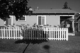
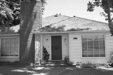
Suburb	0.940		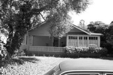		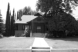	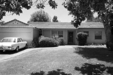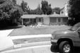InsideCity	Bedroom	Street	InsideCity
InsideCity	0.490					Street	Street	Kitchen	Bedroom
TallBuilding	0.750					Store	Industrial	Bedroom	Street
Street	0.650					InsideCity	Bedroom	InsideCity	TallBuilding
Highway	0.750					Industrial	Street	Suburb	InsideCity
OpenCountry	0.370					Coast	Coast	Coast	Coast
Coast	0.840					Highway	OpenCountry	Mountain	OpenCountry
Mountain	0.870					OpenCountry	TallBuilding	Coast	Industrial
Forest	0.910					Mountain	Mountain	Mountain	Mountain
Category name	Accuracy	Sample training images		Sample true positives		False positives with true label		False negatives with wrong predicted label

Evidently, using a bag of SIFT's along with an SVM lead to the best results. This is likely due to how sensitive 1 nearest neighbor is to noise and outliers. SVM's tends to not be affected as much by outliers. Also KNN's advantages tends to show when there is a much larger dataset. If our dataset was infinitely* large, then KNN would actually perform very well (as long as we used all of the pixels as the features), while SVM would run into issues due to it's lack of expressiveness (it can only find hyperplanes in the feature space, while KNN can find arbitrary decision boundaries). Unfortunately we don't have enough data for these advantages to become apparent.
*note it wouldn't be infinite because there is a finite number of images of a given size.