Project 4 / Scene Recognition with Bag of Words

Image recognition is one of the most fundamental problem in computer vision. The goal of this project is to classify a scene using different machine learning methods with various complexity. Feature Computation i.e. representation of an image as a vector is used to train and test a classifier. Classififers such as nearest neighbour and SVM were trained using tiny images(simple feature method) and bags of quantized local features (advanced feature method) . The following three combinations of image features and classifiers are implemented and analysed

1. Tiny image representation and nearest neighbour classifier
2. Bag of SIFT representation and nearest neighbor classifier
3. Bag of SIFT reprentation and linear SVM classifier

Image Representation and Feature extraction

Tiny Image Representation

In case of tiny image representation, each image is simply resized to a small fixed resolution of 16x16. The images are made to have zero mean and unit length. Since the image is only resized it is not inavriant to spatial and brightness shifts. Below is psuedo code. It was observed that the results are better when zero mean and unit length operations were applied before resizing the image.

image_height = 16;
image_width = 16;
image_size = image_width * image_height;
[N,~] = size(image_paths);
image_feats = zeros(N,image_size);
 
for i = 1:N
    image_read = double(imread(image_paths{i})); % read the image
    image_read = image_read - mean(image_read(:)); % make the image zero mean
    image_read = image_read/std(image_read(:)); % normalize the image 
    image_read = imresize(image_read,[image_width, image_height]); % resize the image
    image_feats(i,:) = imresize(image_read',[1,image_size]); % add it to the image_feats
end

Bag of SIFT Features

A vocabulary of visual words which is required to represent training and testing examples is obtained by sampling SIFT descriptors from the training images, clustering them with kmeans, and then returning the cluster centers, which forms the visual vocabulary. The SIFT features for the testing examples are initially computed and then each local feature is assigned to its nearest cluster center by comparing it with the vocabulary that already exists. A histogram indicating how many times each cluster was used forms the feature representation for each image. The histogram is normalized so that a larger image with more SIFT features will not look very different from a smaller version of the same image. Below is the pseudo code of the implementation

for i =1:N
    I = imread(image_paths{i});
    [~, SIFT_features] = vl_dsift(single(I),'step',3);
    D = vl_alldist2(vocab',single(SIFT_features));
    [~,Index] = min(D);
    histogram = zeros(1,vocab_size);
    for k = 1:size(SIFT_features,2)
        histogram(Index(k)) = histogram(Index(k))+1; % update the histogram of the corresponding bin
    end
    image_feats(i,:) = histogram / sum(histogram);
end

Classification Techniques

Nearest Neighbour Classifier

The nearest neighbour classifier predicts the category of every test image by finding the training image with most similar features. Votes based on 4 nearest neighbours are used as the performance was maximum for the given k parameter.

	D = vl_alldist2(test_image_feats.',train_image_feats.');
k = 4;
[~,I] = sort(D);
I = I(1:k,:);
labels = train_labels(I);
predicted_categories = [];
for i = 1:size(I,2)
   unique_labels = unique( labels(:,i) );
   n_class = length(unique_labels);
   n = zeros( n_class, 1);
   for j = 1:n_class
      n(j) = length(find(strcmp(unique_labels{j}, labels(:,i))));
   end
   [~, index] = max(n);
   predicted_categories = [predicted_categories ; unique_labels(index)];
end

Linear SVM

A hyperplane is obtained by learning the feature space. The feature space is partitioned and test cases are categorized based on which side of the hyperplane they fall on. This function will train a linear SVM for every category and then use the learned linear classifiers to predict the category of every test image. Every test feature will be evaluated with all 15 SVMs as there are 15 categories and the most confident SVM will "win". Linear SVMs performs better compared to nearest neighbour as the classifier is not heavily influenced by frequent visual words especially if they represent smooth pateches or gradients or step edges thereby improving the accuracy

categories = unique(train_labels); 
num_categories = length(categories);
num_train_images = size(train_image_feats, 1);
LAMBDA = 0.000001;
for i = 1:num_categories
    labels = ones(num_train_images,1).*-1;
    labels(strcmp(categories{i},train_labels)) = 1;
    [W,B] = vl_svmtrain(train_image_feats', labels, LAMBDA);
    confidence(:,i) = test_image_feats*W+B;
end
[~, indices] = max(confidence, [], 2);
predicted_categories = categories(indices);
end

Accuracy and Results

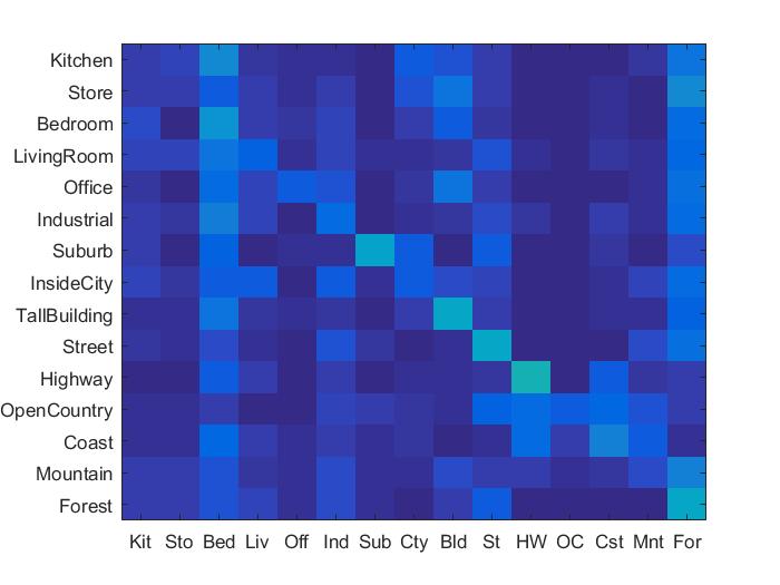
1. Tiny Image Representation and k Nearest Neighbour Classifier

k= 4
Accuracy = 22.2%

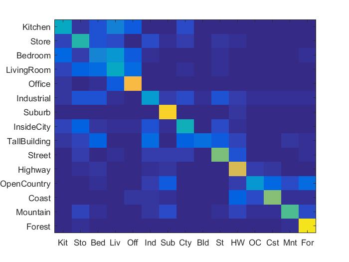
2. Bag of SIFT Features and Nearest Neighbour Classifier

Vocab Size = 400
Accuracy = 53.3%

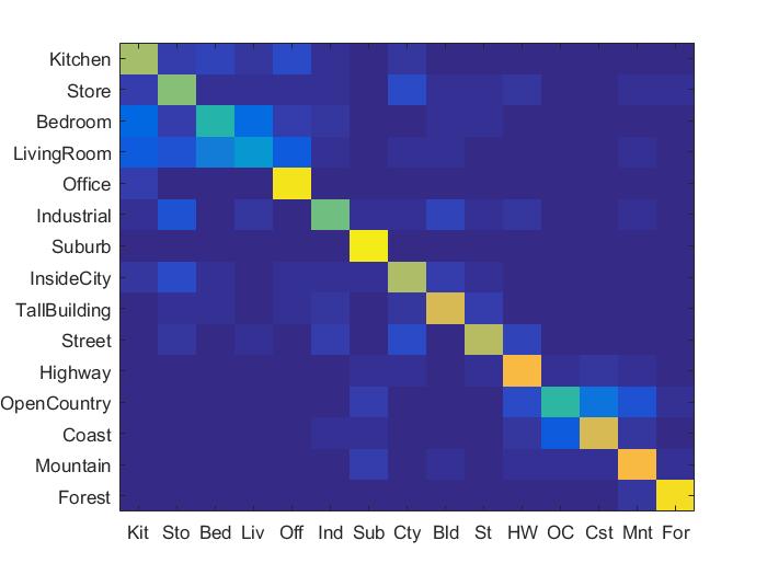
3. Bag of SIFT Features and Linear SVM

Vocab size = 400
Accuracy = 69.7%

Extra Credit

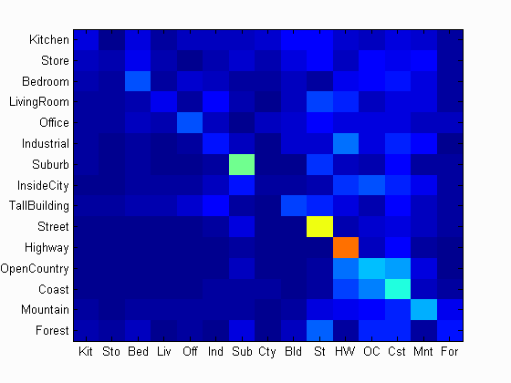
Effect of Vocabulary Size

As can be seen below there is a significant improvement in the performance with the vocabulary size going from 10 to 200 but improves rather slowly for larger vocabulary size. As more clusters are used, the impact of noise and the number of dimension in the feature vector increases.

Scene classification results visualization

Accuracy (mean of diagonal of confusion matrix) is 0.697

Category name	Accuracy	Sample training images		Sample true positives		False positives with true label		False negatives with wrong predicted label
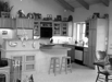
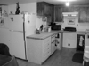
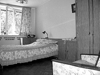
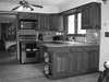
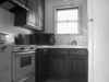
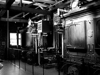
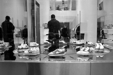
Kitchen	0.670		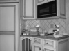			Bedroom	LivingRoom	InsideCity	Bedroom
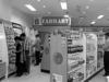
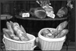
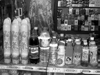
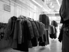
Store	0.600		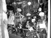			Street	InsideCity	TallBuilding	InsideCity
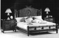
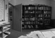
Bedroom	0.430					OpenCountry	Store	Office	LivingRoom
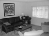
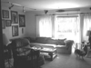
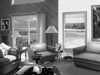
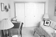
LivingRoom	0.340		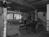			Kitchen	Mountain	Bedroom	Bedroom
Office	0.940					Kitchen	Bedroom	LivingRoom	Kitchen
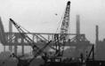
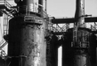
Industrial	0.580					Street	Store	TallBuilding	Store
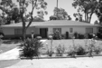
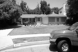
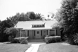
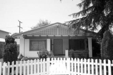
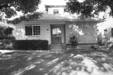
Suburb	0.960		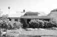			Industrial	OpenCountry	Store	Highway
InsideCity	0.670					TallBuilding	Store	Store	Highway
TallBuilding	0.740					InsideCity	InsideCity	Store	Office
Street	0.690					Bedroom	TallBuilding	Industrial	Store
Highway	0.800					Street	Industrial	Forest	Coast
OpenCountry	0.470					Coast	Highway	TallBuilding	Mountain
Coast	0.790					OpenCountry	OpenCountry	Highway	Mountain
Mountain	0.830					Industrial	Highway	Forest	OpenCountry
Forest	0.940					OpenCountry	Store	Mountain	Suburb
Category name	Accuracy	Sample training images		Sample true positives		False positives with true label		False negatives with wrong predicted label

Conclusion

It is found that the bag of SIFTS feature representation and linear SVM classifier showed higher accuracy. The vocabulary size was varied and a vocab size of 400 was found to give better accuracy without increasing the computation time immensely.