Project 4 / Scene Recognition with Bag of Words

In this project, different methods for scene classification have been explored. Tiny images and bag of words features are used, and then two different classifiers are tried out and the results comapred.

Tiny Image Features with K-Nearest Neighbour

Here, I downsample the image to 16x16 and use the 256 pixels thus obtained as the feature descriptor corresponding to that image. In my code, I first crop the image to make sure its aspect ratio is 1 before resizing to 16x16. After this, I implement the nearest neighbour classifier which assigns to every query image the category of its closest match in the training data. A slight variation involves checking the k closest neighbours and assigning the most occuring category among these neighbours. Using this pipeline, I got an accuracy of 19.5% for a K=4 using the standard distance metric.

Bag of SIFT (Nearest Neighbour + SVM)

Here, I build a bag of sifts model by creating a vocabulary of words. This is done by densely sampling all images in the training set and then using k-means to find a certain number of cluster centres. These centres form the visual words in the vocabulary. The feature for each image is constructed by taking a histogram of the number of occurrences of each visual word in it. For the submission, I use a vocabulary of 200 words. The below image shows the accuracies obtained for the submitted code with the bag of sift model with each of the two classifiers with all extra credit options turned off.

Nearest Neighbour Accuracy: 61.7%	SVM Accuracy: 64.7%

Naive Bayes Nearest Neighbour

I implemented the algorithm described by Boiman et al which does not quantise the descriptors at all, and uses descriptor to class distance to assign categories to query images. The authors claim that the descriptors are sparse and clustering them actually throws away a lot of information. Hence, I implemented the algorithm without quantisation. The biggest challenge, of course, was the sheer number of descriptors whose distances needed to be calculated. Because of this, I heavily increases the 'step' parameter to a value of 20 (values lower than 10 gave me out-of-memory errors).

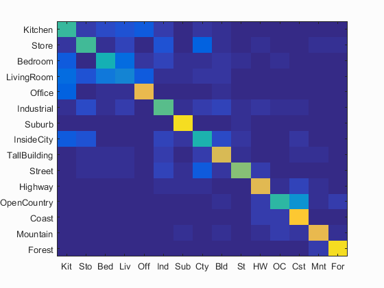
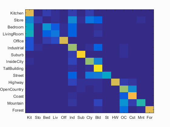
Exact Nearest Neighbour: I tried computing the exact distances (i.e. without using a kd-tree). This took about 4 hours to run on my laptop, but gave me excellent results relative to the step size. I got an accuracy of 60.8% for a step size of 20. In comparison, the normal kNN gave about 43% for the same step size. Below is visualised the confusion matrix for this algorithm, and a kNN run at the same sampling size. Clearly, this method would have done way better given time or a more efficient way of computing distances.

Accuracy: 60.8%	Accuracy: 43.2%

kd-tree: I also implemented the same with the kd-tree. This was about 3 times faster, but gave me a relatively inaccurate result, probably because kd-tree gives approximate nearest neighbours. I have still left this section in the code but it is turned off by default.

Kernel Codebook

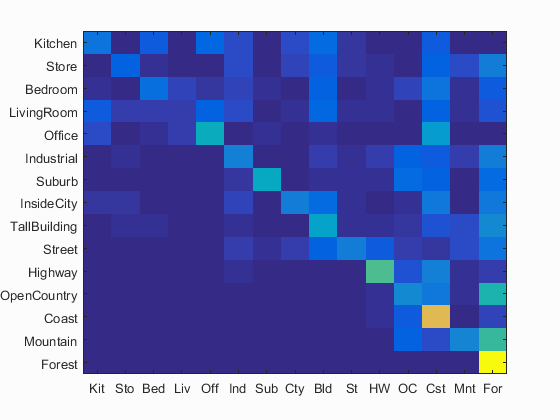
I implemented a soft binning method by adding weights based on the distances to the top four closest visual words. I tried different methods and finally settled by weighting them as r*(1-(di/d1+d2+d3+d4)), where r is maximum for the closest neighbour and grows progressively smaller for the other three. This increased my accuracy for SVM by about 5%, to a value of 69.8% with 'fast' settings and high step size. Here is the confusion matrix of the same:

Fisher Encoding

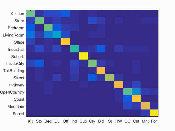
Because vl_gmm takes comparable time to k-means, I also saved the variables it generated. Since this saves the relative position and variance with respect to each cluster centre, we have a feature vector of size N x 128*2*means. I got the best results overall using Fisher encoding. SVM gave me an accuracy of 76.7% for a feature with 100 means. Somewhat interestingly, nearest neighbour was not just slow, but also gave very poor results, probably because of the extreme high dimensionality of each vector.

Because this gave me the best results, I have included the entire confusion matrix and the table generated by the starter code for this case.

Scene classification results visualization

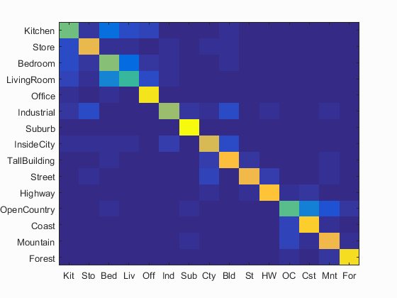
Accuracy (mean of diagonal of confusion matrix) is 0.767

Category name	Accuracy	Sample training images		Sample true positives		False positives with true label		False negatives with wrong predicted label
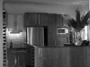
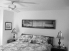
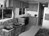
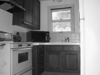
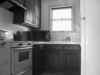
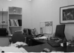
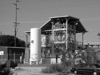
Kitchen	0.590		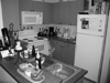			Bedroom	Store	Store	Bedroom
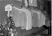
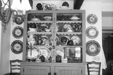
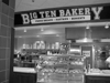
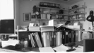
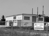
Store	0.790		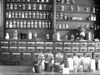			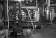Industrial	Industrial	Kitchen	TallBuilding
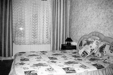
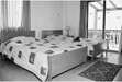
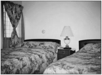
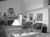
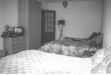
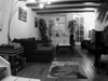
Bedroom	0.610		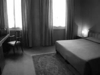			Kitchen	Kitchen	Office	LivingRoom
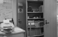
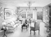
LivingRoom	0.510					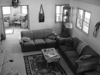Bedroom	Kitchen	Office	Mountain
Office	0.940		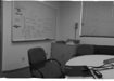			LivingRoom	InsideCity	Kitchen	Kitchen
Industrial	0.650					Bedroom	LivingRoom	Store	TallBuilding
Suburb	0.990		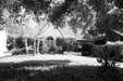			Industrial	Industrial	InsideCity
InsideCity	0.750					TallBuilding	Highway	TallBuilding	Kitchen
TallBuilding	0.830					InsideCity	Industrial	Street	InsideCity
Street	0.810					InsideCity	Forest	InsideCity	Mountain
Highway	0.850					Street	Street	Bedroom	InsideCity
OpenCountry	0.560					Mountain	InsideCity	Coast	Bedroom
Coast	0.890					OpenCountry	Industrial	OpenCountry	OpenCountry
Mountain	0.800					OpenCountry	Forest	Suburb	OpenCountry
Forest	0.930					OpenCountry	OpenCountry	OpenCountry	Street
Category name	Accuracy	Sample training images		Sample true positives		False positives with true label		False negatives with wrong predicted label

Additional Modifications and Observations

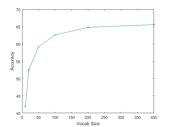
1. Effect of Vocab Size: Quite obviously, the larger the vocabulary size, the higher the accuracy is expected to be. Below is a graph which shows the accuracy for six different vocabulary sizes. It seems to have largely flattened out by the time we reach 400 words, so choosing that as vocabulary size seems to be wasteful. It would merely add to the time heavily because we need to calculate way more cluster means, and not increase the accuracy too much. Hence, in the final code, I have settled for a vocabulary size of 200.
2. Weighted KNN: While doing the knn, instead of taking the mode of k closest categories, I instead went for a weighted approach where I assigned weights based on distances and the category scoring the highest weight was chosen. This actually improved my performance noticeably.For instance, a normal knn without weights with K=7 gave me an accuracy of 60.8, whereas adding weights gave an accuracy of 61.7%.
3. Effect of Varying K in Nearest Neighbour: I have plotted a graph which shows the variation of accuracy with change in K.
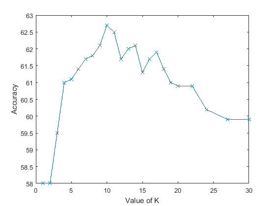
   Again, as expected, the accuracy increases up to a certain value of K and then starts reducing. For this particular set of images, I got my best performance at K=10. Just out of curiosity, I checked the accuracy for K=100 and K=1000 and they were still very reasonable: 56.7% and 42.3%. This was most probably because of the weighted approach I used (K=1000 would actually have some categories fully filled out since we have only 1500 images! So a blind mode-based approach would assign a random category).
4. Effect of Lambda in SVM: This parameter was actually much harder to quantify. Even at the same values of the parameter,multiple runs were yielding slightly varying results. However, for almost all features I tried (kernel codebook, Fisher, NBNN), values of the order of 0.0001 seemed to perform the best.
5. General observation regarding the results: Most algorithms had trouble distinguishing the indoor scenes whereas they did quite well with outdoor scenes (forests, suburbs). The only reason I can think of for this being the case is possibly because of the similarity of sizes of objects contained in the each of the rooms (losing spatial layout makes it all that harder). In contrast, something like a forest seems to have distinctive patterns (trees) which are not found in other classes.