Project 4 / Scene Recognition with Bag of Words

Tiny Images

For each image from the training set, the images were read from the provided paths, then resized to 16x16 using imresize. Then to improve performance, the data has been zero-centered and normalized.

Building Vocabulary + Bag-o-SIFT

In order to get the vocabularies needed for running the bag of sift function, each image from the training set were converted into SIFT features using vl_dsift, then clustered into k centers, where k is the number of vocabulary initially set in the pipeline. Then using the vocabulary, recalculate the sift features for each image and create a histogram of SIFT features. For each SIFT feature, the histogram is incremented to one of the vocabularies with the closest distance (euclidean). Then all of the histograms are normalized before being used as features.

k-Nearest Neighbor

For classification, the k-nearest neighbor was implemented. Given a single feature vector to be classified, the distances from the training features were calculated and then sorted. Then based on the input value k, the top k features were selected to vote. Due to the nature of max function of matlab, the results have bias towards labels mentioned first in the unique function when calculating max.

Linear SVM

Since vl_svmtrain is a linear classifier, the training occured 15 times (total number of scene categories), each with different W and b values. Then using the combined matrix of W's and b's, each test features were evaluated to produce scores for each category. The one with the largest score is set as the category of the image.

Accuracy for each combination

1. kNN = 10, Tiny images: 0.189
2. kNN = 10, Bag-o-sift: 0.513
3. SVM, Tiny images: 0.181
4. SVM, Bag-o-sift: 0.676

Overall, the bag of sift features resulted in better accuracy than using tiny images as features. It's interesting to note that the accuracies when using tiny images as features does not vary depending on either classifier. This could be attributed to the fact that tiny images are weak features for classification tasks. The best results came from using the linear SVM classifier and bag of sift features. Further generated results are shown below. The results were initially around ~0.50 with the same parameters when training with tiny images, but trying various paramter values for lambda and number of iterations in vl_svmtrain improved performance significantly. This signifies the importance of parameter tuning.

Scene classification results visualization

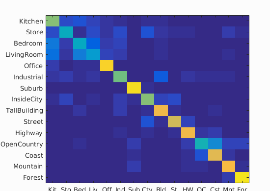
Accuracy (mean of diagonal of confusion matrix) is 0.676

Category name	Accuracy	Sample training images		Sample true positives		False positives with true label		False negatives with wrong predicted label
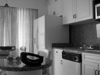
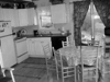
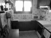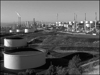
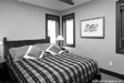
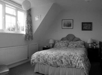
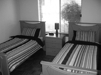
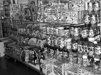
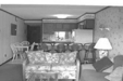
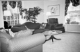
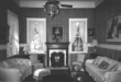
Kitchen	0.620					Industrial	Bedroom	Store	LivingRoom
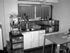
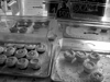
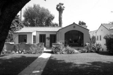
Store	0.420					Mountain	LivingRoom	Forest	TallBuilding
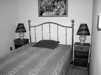
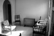
Bedroom	0.400					LivingRoom	LivingRoom	Industrial	Industrial
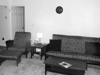
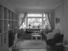
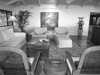
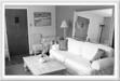
LivingRoom	0.340		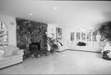			InsideCity	Kitchen	Bedroom	Store
Office	0.900					LivingRoom	LivingRoom	Kitchen	Bedroom
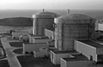
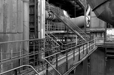
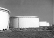
Industrial	0.590					TallBuilding	InsideCity	OpenCountry	Highway
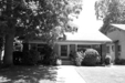
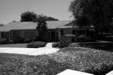
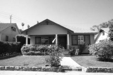
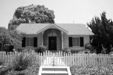
Suburb	0.930		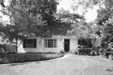			OpenCountry	OpenCountry	Coast	OpenCountry
InsideCity	0.610					Store	Store	TallBuilding	Street
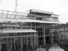
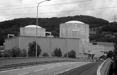
TallBuilding	0.800					Industrial	Industrial	Street	Bedroom
Street	0.740					InsideCity	InsideCity	OpenCountry	Highway
Highway	0.800					Street	Coast	Industrial	Bedroom
OpenCountry	0.450					Highway	Store	Forest	Suburb
Coast	0.780					OpenCountry	OpenCountry	Highway	Mountain
Mountain	0.820					Forest	LivingRoom	OpenCountry	Highway
Forest	0.940					Mountain	Street	Mountain	Mountain
Category name	Accuracy	Sample training images		Sample true positives		False positives with true label		False negatives with wrong predicted label

According to the table results separated into accuracies per category, 'Living Room' had the worst accuracy, followed by bedroom. It seems that many examples of living room had been categorized as living room, and vice versa. It is possible that the sofas in living rooms are confused with the beds in living rooms, as evidenced by the sampled images. The classifier performed best in forest and suburb categories. For forest, the classifier could have looked for complexly textured leaves throughout the image, and for suburbs half grass and half straightly outlined houses. This is because SIFT features are sensitive to orientation of edges and their relative location.

Cross-Validation (EC)

In the cross_validation.m file, the code performs the same as previously done so far, but with smaller training and testing sets(100 each), which are all sampled from the original training set. Using the same parameters mentioned above, the average and the standard deviation results are below. For linear SVM, to save computation time, the same vocab.m extracted from the original 1500 training set.

Accuracy for each combination using CV

1. kNN = 10, Tiny images: MEAN: 0.142, STD: 0.035
2. kNN = 10, Bag-o-sift: MEAN: 0.347, STD: 0.058
3. SVM, Tiny images: MEAN: 0.187, STD: 0.049
4. SVM, Bag-o-sift: MEAN: 0.469, STD: 0.065

Accuracy for each combination

1. kNN = 10, Tiny images: 0.189
2. kNN = 10, Bag-o-sift: 0.513
3. SVM, Tiny images: 0.181
4. SVM, Bag-o-sift: 0.676

With the exception of tiny images with SVM, the mean accuracies are lower than the original 1500. Unlike the previous without CV, the SVM using tiny images performs better than kNN using tiny images. However this could signify that SVM is more invariant to size of the dataset at classifying in comparison to kNN, as evidenced by cross-validation, whereas kNN should vary the k value if the size of the dataset decreases.