Project 4: Scene recognition with bag of words
Introduction
This project's goal was given an image as input, output a string stating the scene of the image. A bag of words approach was used for this scene recognition task. The project has three major components: 1) Feature representation, 2) Classification of image given feature representation, 3) Evaluation of classification. For this project, I implemented parts 1 and 2, and will describe in more detail the steps involved for each part. I will describe the different approaches in parts 1 and 2, the parameter optimization, and how the results are affected by different combinations of parts 1 and 2.
Component 1A: Feature Representation with Tiny Image
I first implemented calculation of the feature representation. This task is similar to the project where the task was to identify interest points in corresponding images using SIFT features. Instead of interest points, we want to create a low dimensional descriptor of the image that describes the image scene. The most basic feature representation that can be used for an image, just like with an interest point, is the image itself. This was the first implementation of the feature representation part. I created tiny image feature representations for each image. I did so by first down-sampling the image to 16x16 (for a total of 256 features in the descriptor), subtracting the mean from the image, and normalizing the image. I did this for all 1500 training images, and 1500 test images.
Component 1B: Feature Representation with Bag of Sifts
Another approach that can be used for feature representation is instead of using the image itself, or a subsection of the image, we instead use a collection of SIFT features to represent the image. This approach of bags of SIFT features makes the assumption that an image's unique characteristics and description of the scene are based on the collection of interest points in the image. This makes intuitive sense in that the corners of an image make up the outline of the image, e.g. the points of mountains are distinctly different from the human made corners in an office setting or building. However, because each image is inherently different and has a unique set of interest points (the union of two mountain images' interest points is most likely empty), we have to cluster similar interest points together and compute cluster average centers of interest points. I used k-means clustering to compute 500 centers of interest points. I used the VL_feat() library to compute SIFT features for each image in the training data set. The parameters I used for VL_feat() for the vocabulary were 'fast' for fast approximation of the Gaussian sliding window, and a step size of two, to get a very dense set of interest points for each image. I had initially made my vocabulary with a subset of images and about 5000 interest points for each image, but using a denser set and all the images resulted in a couple of percentage points increase in accuracy.
Component 2A: Nearest Neighbor Classification
Now that I have covered the two methods for feature representation used for this project's scene classification, I will now discuss the two methods used to classify the scene of an image that has not been seen before. The two classification methods used in this project are k-nearest neighbors classification, and 1 vs. all support vector machine classification. K-nearest neighbors takes in a new test point, "plots" it in a higher dimensional space, and searches for its k-closes training data neighbors using some distance metric. The training data neighbors have associated labels, so they vote on the new test point's label. I implemented an inverse distance weighted k-nearest neighbors, and I found after testing 1, 3, 5, 10, and 20 neighbors that 3 was the optimal parameter for the testing accuracy.
Component 2B: SVM Classification
One other method used for scene classification in this project is one vs. all support vector machines. Support vector machines are linear separators of high dimensional data. Usually, SVM is used for binary classification. To use SVM, we convert the multiclass problem of scene recognition (building, forest, sky) down to a binary task (forest and not forest) for all 15 scene classes in our database. SVM in Matlab returns the projection matrix W and bias b that is the high-dimensional plane that separates the data. The regularization parameter was varied and optimized for improved test-accuracy performance. An optimal lambda was found to be 0.0001. For each test point, all fifteen trained SVM classifiers are applied to the test point and the max value (closest to 1, where 1 means it belongs to that scene class) is taken as the predicted scene label.
Component 3: Evaluation
First, I evaluated a tiny image descriptor with nearest neighbors. First I discuss nearest neighbor parameter manipulation. With one nearest neighbor alone and no distance weighting, an accuracy of 22.5% was obtained. With more neighbors, such as 10, accuracy drops to 21.3%. This is because further away points from the test point have equal voting say in the label of test point. With inverse distance weighting (weight the vote more of a closer point to test point) and 10 neighbors, an accuracy of 23.1% is achieved. Using more neighbors such as 20 with distance weighting, increases accuracy to 23.2%, marginally better. The best distance metric used was standard L2 Euclidean distance, which along with Manhattan are the typical distance metrics used for high-dimensional points. The final implementation, with 10 inverse distance weighted neighbors and using the L2 distance metric, zero-mean and normalized, obtained a test accuracy of 23.1% in 26.2 seconds for the full pipeline. Improving tiny image features with zero-mean and normalization improved accuracy substantially from 20.3% to 23.1%.
Second, I evaluated bag of sift feature descriptor with nearest neighbors. I built the vocabulary as already mentioned above. I obtained sift features for the training and testing data with a step size of five and a bin size of 2, meaning small but sparse features. I obtained this parameter setting via trial and error. For an SVM classification, using bin size of 4 obtained an accuracy of 64%, 8 was 58.3%, 2 is 65.1%. This is interesting because the bin size used to build the vocabulary was 4. To improve performance run time, I stored the 500 clusters from my vocabulary in a KD-tree for fast look up of the closest clusters for each sift feature. The resulting histogram of the vocabulary of the image (how the sift features of an image were distributed across the 500 clusters) was what used later on in nearest-neighbor and SVM classification. The distance metric in nearest neighbors had a huge impact on performance, since the dimensions of each point was based on a value in a histogram bin. Using L2 distance metric achieve an accuracy of 50.9%. Using the HELL distance metric improved accuracy to 53.5%. To improve performance on getting the bags of sift features, I used a step size of 6. The overall implementation took 555.23 seconds on my computer.
Third, I evaluated the bag of sift feature descriptor with SVM. As mentioned above, the best SVM classification run obtained an accuracy of 65%. Hyperparameters for bag of sifts was maintained, and as mentioned before the best lambda used was 0.001 for regularization. The overall implementation took 542.88 seconds on my computer. All three pipelines are under 10 minutes.
Component 5: Conclusion
Conclusion: By first performing feature representation of the images using either a tiny images descriptor or a bag of sifts feature vector and classifying using either k-nearest neighbors or support vector machine, this project demonstrates an implementation of scene recognition.
Component 5: Results Webpage
Scene classification results visualization
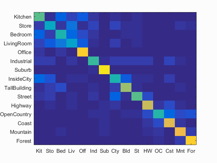
Accuracy (mean of diagonal of confusion matrix) is 0.630
| Category name | Accuracy | Sample training images | Sample true positives | False positives with true label | False negatives with wrong predicted label | ||||
|---|---|---|---|---|---|---|---|---|---|
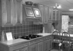
| Kitchen | 0.550 | 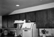 |
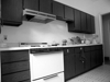 |
 |
 |
 Bedroom |
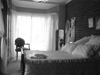 Bedroom |
 InsideCity |
 Bedroom |
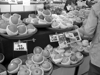
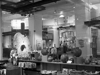
| Store | 0.400 |  |
 |
 |
 |
 LivingRoom |
 InsideCity |
 LivingRoom |
 Kitchen |
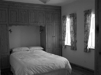
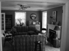
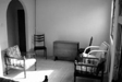
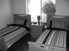
| Bedroom | 0.460 |  |
 |
 |
 |
 LivingRoom |
 LivingRoom |
 Suburb |
 Store |
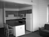
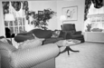
| LivingRoom | 0.370 | 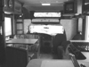 |
 |
 |
 |
 Store |
 Store |
 Kitchen |
 Bedroom |
| Office | 0.890 |  |
 |
 |
 |
 LivingRoom |
 Bedroom |
 Bedroom |
 Bedroom |
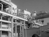
| Industrial | 0.510 | 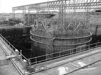 |
 |
 |
 Mountain |
 Bedroom |
 Store |
 Kitchen |
|
| Suburb | 0.940 |  |
 |
 |
 |
 Highway |
 Mountain |
 Store |
 Industrial |
| InsideCity | 0.460 |  |
 |
 |
 |
 Store |
 Highway |
 TallBuilding |
 Kitchen |
| TallBuilding | 0.650 |  |
 |
 |
 |
 InsideCity |
 InsideCity |
 Coast |
 Bedroom |
| Street | 0.560 |  |
 |
 |
 |
 OpenCountry |
 Bedroom |
 Store |
 Highway |
| Highway | 0.720 |  |
 |
 |
 |
 Street |
 Coast |
 InsideCity |
 Store |
| OpenCountry | 0.480 |  |
 |
 |
 |
 Highway |
 Coast |
 Mountain |
 Coast |
| Coast | 0.770 |  |
 |
 |
 |
 InsideCity |
 OpenCountry |
 Highway |
| Mountain | 0.800 |  |
 |
 |
 |
 Forest |
 OpenCountry |
 Highway |
 LivingRoom |
| Forest | 0.890 |  |
 |
 |
 |
 Store |
 Mountain |
 OpenCountry |
 Coast |
| Category name | Accuracy | Sample training images | Sample true positives | False positives with true label | False negatives with wrong predicted label | ||||