Project 4 / Scene Recognition with Bag of Words

Feature Representations:

1. Tiny Images

   Tiny images are a very simple image descriptor where we simply downsize the image to 16 × 16 and flatten it by using the reshape function in MATLAB to give a 256 dimensional feature representation for the image.

2. Bag of sifts

   Here the goal is to build vocabulary of visual words from SIFT descriptors and then features are generated by classifying each SIFT descriptor to one of the visual word based on the distance. We build a histogram of counts of assignments to each visual word which is then used as the feature vector for that image. Basically, I'm building the vocabulary for each image at a step size of 32 and a bin size of 16, I calculate the SIFT descriptors using the vl_dsift method. Then out of all the SIFT descriptors calculated I randomly pick 100 of them and append it to my 'features' matrix. Then using the vl_kmeans function we can get the k (= 200) centroids which represents our vocab matrix. This is a computationally intensive procedure and the vocab matrix is saved to be used further. In get bags of sifts the procedure is similar. The only difference is that I am doing an even denser SIFT descriptor calculation i.e. with step size of 4 and the same bin size of 16 albeit using the 'fast' parameter of vl_dsift and then preparing a histogram of counts of points assigned to each cluster.

3. Gaussian Pyramid (Graduate/Extra credit)

   Here we use the same idea as before with the only difference that we repeat the procedure at multiple levels of Gaussian Pyramid i.e. we smooth the image using a Gaussian kernel and downsize it to ^m⁄₂ × ⁿ⁄₂ every time given m × n is the original dimensionality of the image.

4. Spatial Pyramid (Graduate/Extra credit)

   This method is an improvement over the vanilla bag of sifts method. Basically, here we consider the SIFT descriptors at multiple levels. At level 0 the coarsest level we are considering the entire image which is same as the bag of sifts method. At level 1 the image is divided into 4 quadrants and a histogram is constructed for each quadrant. To construct a histogram for a quadrant only the SIFT descriptors for that particular quadrant are considered. Here we will have 4 quadrants. Similarly, for level 2 we will have 16 quadrants and we will get 16 histograms. We also weigh the counts by the level number i.e. we divide the counts by 2^{L - ℓ} where ℓ = 0, 1, 2 and L = 3. The idea is that at the finer level the SIFT descriptors belonging to same cluster better represent the image as opposed to the coarser level. Therefore, at coarser level we divide the counts by a larger number. We normalize the feature vector later on for each image. As an addition dimensionality reduction techniques like PCA, LDA, pLSA etc. to reduce the computational load at the expense of accuracy.

5. Gist descriptors and Self-similarity descriptors (Graduate/Extra credit)

   Here, in addition to bag of sifts we also make use of gist and self-similarity descriptors. In case of self-similarity descriptors we need to carry out a similar procedure like build vocabulary. Specifically, we will do log polar binning for patch size of 5 × 5, radius of 40, dividing into 3 sectors and then an angular division into 12 parts each. Therefore, we will have number of 36 dimensional self-similarity descriptors out of which we will build a vocabulary by doing k-means. During feature generation then we will buikd a histogram based on counts of cluster assignments.

6. Fisher vectors

   Instead of using k-means we can use Gaussian mixture model and then save the means, covariances and priors. These matrices can then be used to calculate fisher vectors from the SIFT descriptors of an image. These are very powerful features and give the maximum accuracy among all the methods.

Classification:

1. k Nearest Neighbors

   In this method we simply find the k nearest neighbors for each test image feature vector and the predicted category is determined by majority voting. There is a free parameter k to work with.

2. Multiclass SVM

   Here we train a binary SVM classifier for each category wherein we considered everything not in this category as belonging to negative class. Here we have a free parameter lambda which controls the regularization and the accuracy of the model is sensitive to the value of this parameter.

Results

Tiny images and kNN

k	Accuracy (%)
1	22.5
10	23.7
20	22.0
50	20.9

Bag of sift and kNN

k	Step Size	Bin Size	Accuracy (%)
1	2	8	48.2
10	2	8	49.1
20	2	8	47.9
1	4	8	48.2
10	4	8	49.5
20	4	8	48.7
1	2	16	48.7
10	2	16	49.3
20	2	16	49.1
1	4	16	47.5
10	4	16	49.7
20	4	16	48.5

Bag of sift and SVM

lambda	Step Size	Bin Size	Accuracy (%)
0.000001	2	8	66.1
0.000005	2	8	68.0
0.00001	2	8	67.6
0.00005	2	8	63.3
0.000001	4	8	66.0
0.000005	4	8	66.1
0.00001	4	8	66.5
0.00005	4	8	62.9
0.000001	2	16	62.1
0.000005	2	16	67.6
0.00001	2	16	66.0
0.00005	2	16	65.9
0.000001	4	16	61.5
0.000005	4	16	63.7
0.00001	4	16	63.5
0.00005	4	16	62.4

Spatial Pyramid (3 levels) and SVM

lambda	Step Size	Bin Size	Accuracy (%)
0.000001	4	16	70.1
0.000005	4	16	70.7
0.00001	4	16	68.0
0.00005	4	16	66.3

Gaussian Pyramid (2 levels) and SVM

lambda	Step Size	Bin Size	Accuracy (%)
0.000001	4	16	67.1
0.000005	4	16	65.4
0.00001	4	16	63.0
0.00005	4	16	60.9

Bag of sift + GIST and SVM

lambda	Step Size	Bin Size	Accuracy (%)
0.000001	4	16	67.9
0.000005	4	16	67.7
0.00001	4	16	63.0
0.00005	4	16	60.2

The self-similarity descriptors may work much better however, time constraint prevented me from experimenting with it. With the default settings it takes approx 37 seconds to calculate self-similarity descriptors for an image. Increasing patch size, descriptor radius and decreasing number of angular divisions within each sector I could get it down to 10 seconds per image but even this was prohibitive to run through all 3000 images.

Fisher vectors

lambda	Accuracy (%)
0.000001	71.6
0.000005	73.2
0.00001	70.9
0.00005	70.1

Cross-Validation

I attempted cross-validation wherein I take 100 samples per class with replacement for each of train and test set. Following are average accuracy and standard deviation observed over different number of iterations (Considering lambda = 0.000005, step size = 4 and bin size = 16 for bag of sifts:

iters	Avg. accuracy (%)	Standard deviation
1	59.5	0.19
2	60.8	0.18
5	59.7	0.14
10	60.34	0.14

Varying dictionary size (using bag of sifts and SVM)

Dictionary size	Accuracy (%)
10	51.9
20	60.8
50	61.7
100	65.34
200	68.0
500	69.34
1000	66.0

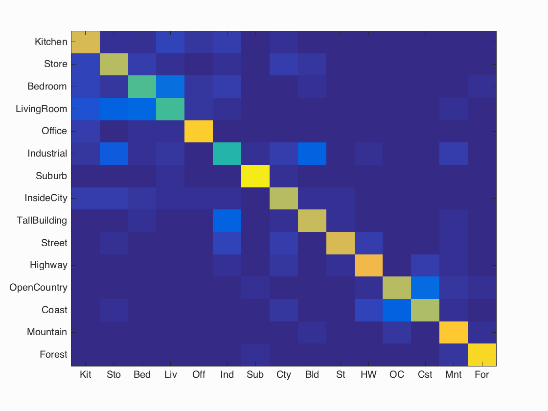
Scene classification results visualization

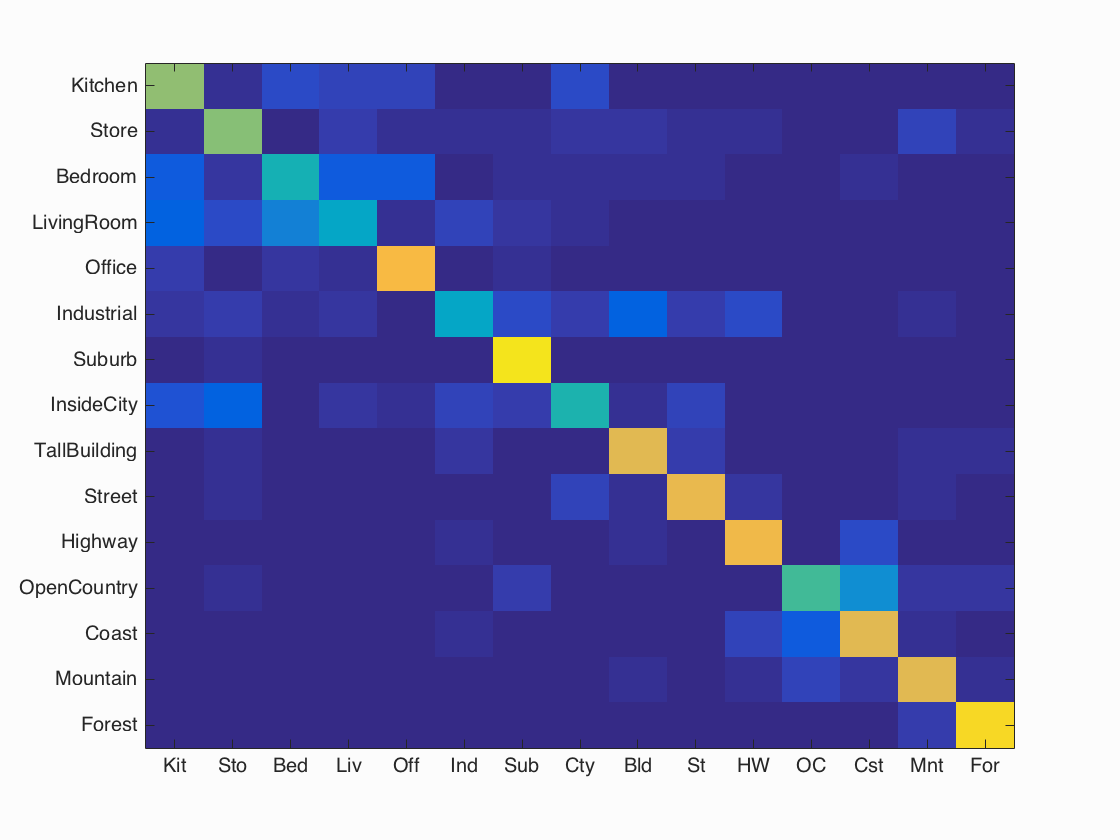
Best performing method (not graduate/extra credit): Bags of sifts + SVM (lambda = 0.000005)
Accuracy (mean of diagonal of confusion matrix) is 0.671

Category name	Accuracy	Sample training images		Sample true positives		False positives with true label		False negatives with wrong predicted label
Kitchen	0.630					LivingRoom	LivingRoom	Bedroom	InsideCity
Store	0.610					InsideCity	InsideCity	Coast	LivingRoom
Bedroom	0.450					Industrial	Office	OpenCountry	Office
LivingRoom	0.380					Bedroom	Kitchen	Suburb	InsideCity
Office	0.820					Kitchen	Store	Industrial	Bedroom
Industrial	0.380					Suburb	InsideCity	Office	Store
Suburb	0.950					LivingRoom	Street	Forest	Industrial
InsideCity	0.460					Street	Street	Store	Kitchen
TallBuilding	0.780					Industrial	Bedroom	Forest	Store
Street	0.790					Industrial	TallBuilding	Mountain	TallBuilding
Highway	0.810					Industrial	Street	Coast	Forest
OpenCountry	0.530					Coast	Coast	Street	Forest
Coast	0.770					OpenCountry	OpenCountry	Highway	Industrial
Mountain	0.780					Coast	Store	Coast	Coast
Forest	0.920					Mountain	TallBuilding	Mountain	Mountain
Category name	Accuracy	Sample training images		Sample true positives		False positives with true label		False negatives with wrong predicted label

Scene classification results visualization

Best performing method: Fisher vector + SVM (lambda = 0.000005)
Accuracy (mean of diagonal of confusion matrix) is 0.732

Category name	Accuracy	Sample training images		Sample true positives		False positives with true label		False negatives with wrong predicted label
Kitchen	0.750					Store	Office	LivingRoom	Bedroom
Store	0.700					Mountain	Kitchen	Kitchen	Industrial
Bedroom	0.540					Industrial	LivingRoom	Industrial	Industrial
LivingRoom	0.530					Bedroom	Bedroom	Bedroom	Store
Office	0.890					Kitchen	LivingRoom	Kitchen	Bedroom
Industrial	0.470					TallBuilding	TallBuilding	LivingRoom	LivingRoom
Suburb	0.960					Industrial	TallBuilding	InsideCity	LivingRoom
InsideCity	0.700					Coast	Highway	Industrial	Kitchen
TallBuilding	0.720					Store	Street	Industrial	InsideCity
Street	0.750					Highway	TallBuilding	Highway	Mountain
Highway	0.810					Street	Street	InsideCity	Mountain
OpenCountry	0.700					InsideCity	Highway	Coast	Suburb
Coast	0.680					OpenCountry	OpenCountry	Mountain	Highway
Mountain	0.870					LivingRoom	OpenCountry	Coast	Forest
Forest	0.910					Bedroom	Mountain	Mountain	Mountain
Category name	Accuracy	Sample training images		Sample true positives		False positives with true label		False negatives with wrong predicted label