Project 4: Scene Recognition with Bag of Words
The objective of this project is to classify scenes in images according to their types. To this end, we either represent these images using the tiny images approach and classify them using K-nearest neighbors (KNN), or sample SIFT features from each image and first build a vocabulary of visual words using K-means, and then construct feature vectors by using the histogram approach where each sampled SIFT feature vector votes for the bin corresponding to the visual word "closest" to it, so that we would have a feature vector corresponding to each photo. For the latter approach, the feature vectors can be classified either using KNN or linear Support Vector Machines (SVM). A list of MATLAB functions implemented are listed below, in the order that they were implemented:
- get_tiny_images.m: This function resizes each image to a small fixed resolution, and enforces each image to have zero mean and unit length.
- nearest_neighbor_classify.m: This is the implementation of the K-nearest neighbors algorithm. The K nearest neighbors of each image feature is returned is labelled by the one with the highest frequency. Note that the value of K must be changed inside the code itself. For optimality, we fix K=5.
- build_vocabulary.m: This function build a vocabulary of visual words by sampling SIFT descriptors from each image, concatenating them, and then perform K-means on them to return the desired number of visual words.
- get_bags_of_sifts: This function computes a feature vector for each image by using the histogram approach where each sampled SIFT feature vector of the image votes for the bin corresponding to the visual word "closest" to it. The histogram is then normalized and then serves as the feature vector.
- get_bags_of_sifts_w_kernel_codebook_encoding.m: This is the extra credit implementation of get_bags_of_sifts.m so that each sampled SIFT feature vector contributes a certain weight to each bin depending on its distance to their corresponding visual word, instead of only voting for the bin corresponding to the word "closest" to it. The gaussian kernel is used, following Chatfield et al.
- svm_classify.m: This is the implementation of the Support Vector Machine classifier. It sets up binary labels of -1 and 1 so that we could make use of the SVM algorithm implemented in VLFeat.
- get_sift_feats.m: This function returns the unquantized SIFT descriptors for use in Naive Bayes Near Neighbor classification. It is used in the starter code as FEATURE='sift'.
- naive_bayes_nearest_neighbor_classify.m: This is the extra credit implementation of the Naive Bayes Nearest Neighbor classifier, following Boiman et al.
- proj4.m : This is the code used to run the project.
Code for Kernel Codebook Encoding
The key part of the code is given below. The only part in which it differs from get_bags_of_sifts is the way in which histograms are voted. With Keneral Codebook Encoding, a sampled SIFT feature vector would vote for every bin of the histogram, with a weight inversely proportional to the distance to its corresponding visual word. Note that we have the down-scale the size of all elements in the Distance matrix, since each element is of the order 10^5, so that using the gaussian kernel with exp(10^5) would result in a number too large to be recognized by MATLAB. It should also be noted that accuracies are highly sensitive to the value of gamma, but I guess this makes sense since scaling using gaussian kernel is highly nonlinear.
     Dist=vl_alldist2(single(feats),vocab');

     Dist=1/10^4*Dist; %rescaling since matrix entries are too large
     Dist=exp(-gamma/2*Dist); %gaussian kernel
     kernel_sum=sum(Dist'); %each column is the sum of each row in Dist

     for j=1:size(feats,2)
         histogram=histogram+Dist(j,:)/kernel_sum(j); %weight contribution to each bin
     end
Results
The accuracies of various Tiny Images/KNN, Bag of SIFT/KNN, and Bag of SIFT/SVM runs are listed below, along with some parameters. Note that the accuracies for SVM were obtained by averaging the result from 10 trials. The visual vocabulary of different sizes (from 10-10000) are saved in the format vocabN.m where N is the number of visual words. The number can be removed when using that vocabulary to run the project. It should be mentioned that the visual vocabulary of size 10000 took over 5 hours to generate; Kmeans seemed extremely slow in converging.
- Tiny Images/KNN, K=1, accuracy = 20%
- Tiny Images/KNN, K=2, accuracy = 20%
- Tiny Images/KNN, K=3, accuracy = 21.7%
- Tiny Images/KNN, K=4, accuracy = 21.5%
- Tiny Images/KNN, K=5, accuracy = 21.9%
- Tiny Images/KNN, K=6, accuracy = 21.6%
- Tiny Images/KNN, K=7, accuracy = 22.7%
- Tiny Images/KNN, K=8, accuracy = 22.3%
- Tiny Images/KNN, K=9, accuracy = 22.6%
- Tiny Images/KNN, K=10, accuracy = 22.9%
- Tiny Images/KNN, K=15, accuracy = 22.9%
- Tiny Images/KNN, K=20, accuracy = 22.4%
- Tiny Images/KNN, K=100, accuracy = 19.1%
- Tiny Images/KNN, K=500, accuracy = 12.7%
- Bag of SIFT/KNN, step size=8, K=1, vocab size = 200, accuracy = 50.3%
- Bag of SIFT/KNN, step size=8, K=3, vocab size = 200, accuracy = 51.2%
- Bag of SIFT/KNN, step size=8, K=5, vocab size = 200, accuracy = 52.1%
- Bag of SIFT/KNN, step size=8, K=7, vocab size = 200, accuracy = 51.3%
- Bag of SIFT/KNN, step size=8, K=10, vocab size = 200, accuracy = 52.7%
- Bag of SIFT/KNN, step size=8, K=15, vocab size = 200, accuracy = 51.1%
- Bag of SIFT/SVM, step size=8, SVM lambda=0.001, vocab size = 10, accuracy = 32.3%
- Bag of SIFT/SVM, step size=8, SVM lambda=0.001, vocab size = 20, accuracy = 45.9%
- Bag of SIFT/SVM, step size=8, SVM lambda=0.001, vocab size = 50, accuracy = 55.8%
- Bag of SIFT/SVM, step size=8, SVM lambda=0.001, vocab size = 100, accuracy = 60.5%
- Bag of SIFT/SVM (with kernel codebook encoding), step size=8, SVM lambda=0.001, vocab size = 200, accuracy = 62.1%
- Bag of SIFT/SVM, step size=8, SVM lambda=0.001, vocab size = 200, accuracy = 62.9%
- Bag of SIFT/SVM, step size=8, SVM lambda=0.0007, vocab size = 200, accuracy = 63.6%
- Bag of SIFT/SVM, step size=8, SVM lambda=0.0005, vocab size = 200, accuracy = 63.6%
- Bag of SIFT/SVM, step size=8, SVM lambda=0.0001, vocab size = 200, accuracy = 61.5%
- Bag of SIFT/SVM, step size=8, SVM lambda=0.001, vocab size = 400, accuracy = 65.0%
- Bag of SIFT/SVM, step size=8, SVM lambda=0.0007, vocab size = 400, accuracy = 65.9%
- Bag of SIFT/SVM, step size=8, SVM lambda=0.0005, vocab size = 400, accuracy = 65.2%
- Bag of SIFT/SVM, step size=8, SVM lambda=0.0001, vocab size = 400, accuracy = 63.2%
- Bag of SIFT/SVM, step size=8, SVM lambda=0.001, vocab size = 500, accuracy = 65.7%
- Bag of SIFT/SVM, step size=8, SVM lambda=0.001, vocab size = 1000, accuracy = 66.3%
- Bag of SIFT/SVM, step size=8, SVM lambda=0.0007, vocab size = 1000, accuracy = 66.1%
- Bag of SIFT/SVM, step size=8, SVM lambda=0.0005, vocab size = 1000, accuracy = 66.0%
- Bag of SIFT/SVM, step size=8, SVM lambda=0.0001, vocab size = 1000, accuracy = 65.4%
- Bag of SIFT/SVM, step size=8, SVM lambda=0.001, vocab size = 10000, accuracy = 69.0%
Observations
Increasing vocabulary size increases the accuracy. Apparently, the limit at which this ceases to occur extends beyond the size of 10000. Also, the lambda parameter in SVM seems to work best with values in the range 0.0005-0.001. Reducing step sizes can lead to better accuracies, since more points are sampled and Kmeans would be more likely to converge to the 'true' center.
Extra Credit
The following extra credit attempts were made.
- Experiment with features at multiple scales (by varying step size to change resolution)
- Implementation of the 'kernel codebook encoding' by Chatfield et al. This leads to an accuracy ~60%, with gamma=1 in the gaussian kernel.
- Performance with different vocabulary sizes, as reported above
- Implementation of the Naive Bayes Nearest Neighbor classifier. By increasing the sample size in get_sift_feats.m, we can get the accuracy to pretty high at the cost of computational time due to the curse of dimensionality. Sampling 25-75 SIFT features for each image and using Naive Bayes NN leads to accuracy ~30%. In a more realistic run, at least 500 features should be extracted, but this wasn't attempted due to the computational time.
Scene classification results visualization
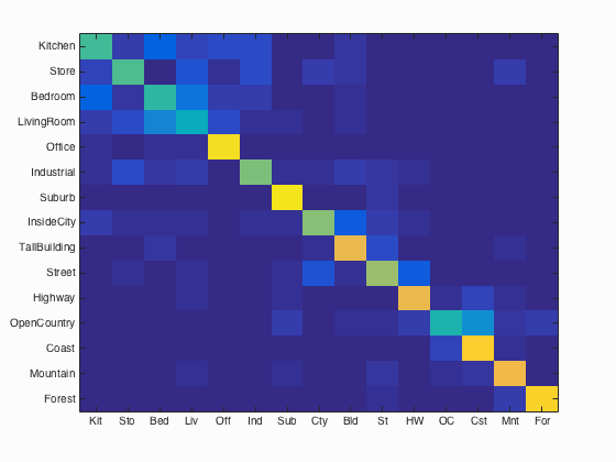
Accuracy (mean of diagonal of confusion matrix) is 0.690
| Category name | Accuracy | Sample training images | Sample true positives | False positives with true label | False negatives with wrong predicted label | ||||
|---|---|---|---|---|---|---|---|---|---|
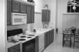
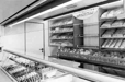
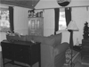
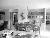
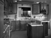
| Kitchen | 0.520 | 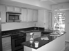 |
 |
 |
 |
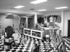
 Store |
 TallBuilding |
 TallBuilding |
 Bedroom |
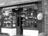
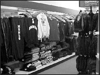
| Store | 0.540 | 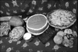 |
 |
 |
 |
 InsideCity |
 LivingRoom |
 LivingRoom |
 LivingRoom |
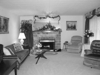
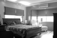
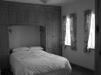
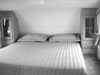
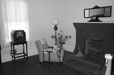
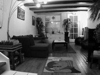
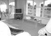
| Bedroom | 0.490 | 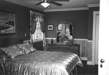 |
 |
 |
 |
 LivingRoom |
 Industrial |
 TallBuilding |
 TallBuilding |
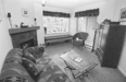
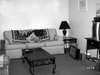
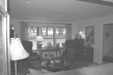
| LivingRoom | 0.420 |  |
 |
 |
 |
 Kitchen |
 Mountain |
 TallBuilding |
 Office |
| Office | 0.930 | 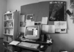 |
 |
 |
 |
 LivingRoom |
 Bedroom |
 LivingRoom |
 LivingRoom |
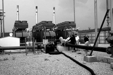
| Industrial | 0.600 |  |
 |
 |
 |
 Bedroom |
 Kitchen |
 Kitchen |
 Store |
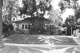
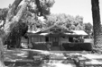
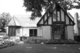
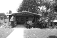
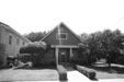
| Suburb | 0.950 | 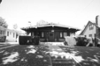 |
 |
 |
 |
 Forest |
 LivingRoom |
 Street |
 Street |
| InsideCity | 0.610 |  |
 |
 |
 |
 Store |
 Street |
 Kitchen |
 Highway |
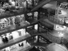
| TallBuilding | 0.790 |  |
 |
 |
 |
 Kitchen |
 InsideCity |
 Bedroom |
 InsideCity |
| Street | 0.650 |  |
 |
 |
 |
 Suburb |
 Mountain |
 Highway |
 Industrial |
| Highway | 0.790 |  |
 |
 |
 |
 OpenCountry |
 InsideCity |
 Coast |
 OpenCountry |
| OpenCountry | 0.460 |  |
 |
 |
 |
 Coast |
 Coast |
 Mountain |
 Forest |
| Coast | 0.890 |  |
 |
 |
 |
 OpenCountry |
 OpenCountry |
 OpenCountry |
| Mountain | 0.810 |  |
 |
 |
 |
 Coast |
 Store |
 Coast |
 Street |
| Forest | 0.900 |  |
 |
 |
 |
 Store |
 OpenCountry |
 Street |
 TallBuilding |
| Category name | Accuracy | Sample training images | Sample true positives | False positives with true label | False negatives with wrong predicted label | ||||