Project 4 / Scene Recognition with Bag of Words
Pipeline 1: Tiny Image Features and Nearest Neighbor Classifier
This was a fairly straightforward pipeline to implement. To create the features, I simply resized each image to a 16x16 resolution. For the nearest neighbor classifier, I used the single nearest neighbor (1-NN algorithm). The accuracy that I got was 19.1%, which was close to triple the performance of random chance, and within the parameters specified by the project guidelines. This whole pipeline runs in roughly 2 minutes. The confusion matrix is shown below. It looks like the algorithm tended to guess the "outdoor" images more than others.

Pipeline 2: Bag of Sift Features and Nearest Neighbor Classifier
In this section, the bag of words model was implemented. First, I implemented the vocabulary builder. This section took the sift features from the training images (using a step size parameter of 3, for better accuracy) and clustered them together to create the words. I stuck with the default 200 words for the vocabulary size. Getting the bags of words for each image was probably the most complicated piece of the project. First, my code finds the sift feature in a test image, it then determines which word that feature most closely resembles (similarly to how the nearest neighbor algorithm itself operates), and then creates a normalized histogram of word frequency. I used a step size of 16 here on my best run (smaller step sizes took far too long to run, while large step sizes were less accurate - for example, a step size of 100 led to an accuracy of less than .2), which produced an accuracy of .417. The run time was around 35 minutes.

Pipeline 3: Bag of Sift Features and 1-Vs.-All Linear SVM Classifier
The new piece of implementation for the third pipeline was the SVM classifier. Since the SVM was a binary classifier, there needed to be 15 of them - one for each category with a "yes" or "no" label. Through experimentation, I arrived at a lambda of .000001. This classifier increased performance to .476, again with a run time of around 35 minutes. The results are listed at the bottom of this page. This pipeline also performed better on the outdoor images. For example, it guessed forest correctly 83% of the time.
Conclusion
I was disappointed that I wasn't able to get my metrics (run-time and accuracy) within the parameters outlined in the project description. The run times were what held me back, as I wasn't able to experiment with parameters as much as I would've liked too (although I was able to do this to some extent). The accuracies, however, were directionally correct. I was surprised that the perfomance was even this high though, and I enjoyed this look at the foundations of combining computer vision and machine learning.
Scene classification results visualization
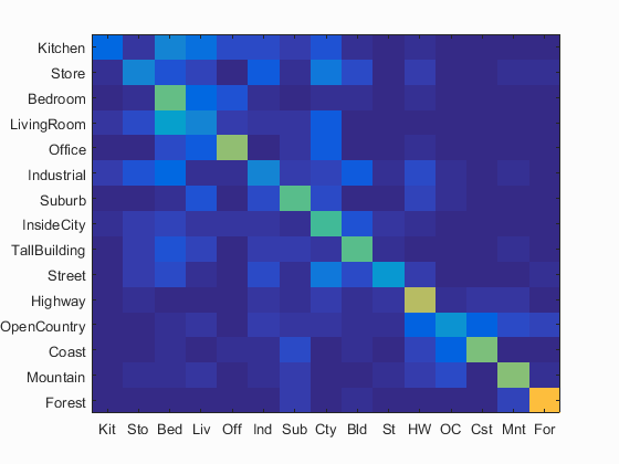
Accuracy (mean of diagonal of confusion matrix) is 0.476
| Category name | Accuracy | Sample training images | Sample true positives | False positives with true label | False negatives with wrong predicted label | ||||
|---|---|---|---|---|---|---|---|---|---|
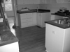
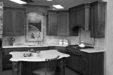
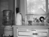
| Kitchen | 0.150 |  |
 |
 |
 |
 Industrial |
 Industrial |
 LivingRoom |
 Mountain |
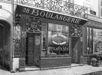
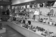
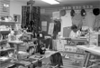
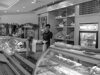
| Store | 0.260 |  |
 |
 |
 |
 LivingRoom |
 Industrial |
 Industrial |
 Suburb |
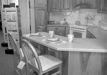
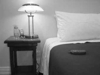
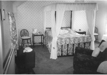
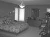
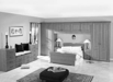
| Bedroom | 0.570 | 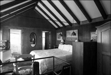 |
 |
 |
 |
 Kitchen |
 Kitchen |
 LivingRoom |
 LivingRoom |
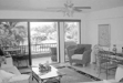
| LivingRoom | 0.260 |  |
 |
 |
 |
 Bedroom |
 Bedroom |
 Bedroom |
 Office |
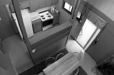
| Office | 0.640 |  |
 |
 |
 |
 Bedroom |
 LivingRoom |
 LivingRoom |
 LivingRoom |
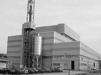
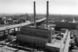
| Industrial | 0.260 |  |
 |
 |
 |
 Kitchen |
 TallBuilding |
 Bedroom |
 Highway |
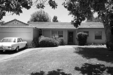
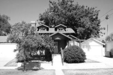
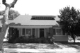
| Suburb | 0.550 |  |
 |
 |
 |
 Coast |
 LivingRoom |
 Store |
 LivingRoom |
| InsideCity | 0.530 |  |
 |
 |
 |
 Store |
 Kitchen |
 Office |
 Kitchen |
| TallBuilding | 0.560 |  |
 |
 |
 |
 Store |
 InsideCity |
 InsideCity |
 Store |
| Street | 0.320 |  |
 |
 |
 |
 TallBuilding |
 Highway |
 Kitchen |
 Suburb |
| Highway | 0.690 |  |
 |
 |
 |
 Mountain |
 OpenCountry |
 Coast |
 Mountain |
| OpenCountry | 0.310 |  |
 |
 |
 |
 Coast |
 Suburb |
 Street |
 Highway |
| Coast | 0.600 |  |
 |
 |
 |
 OpenCountry |
 OpenCountry |
 OpenCountry |
 Suburb |
| Mountain | 0.610 |  |
 |
 |
 |
 OpenCountry |
 OpenCountry |
 OpenCountry |
 OpenCountry |
| Forest | 0.830 |  |
 |
 |
 |
 OpenCountry |
 Street |
 TallBuilding |
 Mountain |
| Category name | Accuracy | Sample training images | Sample true positives | False positives with true label | False negatives with wrong predicted label | ||||