Project 4 / Scene Recognition with Bag of Words

Figure of image recognition
The goal of this project is to implement the image recognition. The process includes two parts, image representation and classifier. There are two types of image representation, tiny images and bags of quantized SIFT features. At the mean time, two different classifiers are nearest neighbor and 1-vs-all linear SVM.
In this assignment, I test three combinations of image representation form and classifier technique, tiny images with nearest neighbor, bags of SIFT features with nearest neighbor and bags of SIFT features with 1-vs-all linear SVM.
Progarm Description
get_tiny_images.m
It is a function to implement the tiny images representations. The tiny images representation is created by simply resizing the image to a smaller, fixed size (e.g. 16x16), and representing this smaller image as a vector.
nearest_neighbor_classify.m
It is a function to implement the nearest neighbor classify images representations. In this function, first, find the distance between each pairs of the test image and the train image, then find the "nearest" train image to the test image, assign the category of train image to the test image
To increase the accuracy, it is need to consider several train images which is close to the test image. And then count the number of category that each train image is in. Assign the category with the most count to the test image. After experiment, K is adjusted to 11 to get the best performance.
Code
for i = 1:M
    for j = 1:N
        D(i,j)=vl_alldist2(test_image_feats(i,:)',train_image_feats(j,:)');
    end
%%%%%%%% k=1 %%%%%%%%%%
     [~,I]=min(D(i,:));
     predicted_categories{i} = train_labels{I};
%%%%%%%% k>1 %%%%%%%%%%
    K = 11;
    tmp = sort(D(i,:),'ascend');
    indice = find(D(i,:)<=tmp(K));
    count = zeros(1,K);
    for k = 1:K
        for k2 = 1:K
            count(1,k)=count(1,k)+strcmp(train_labels{indice(k)},train_labels{indice(k2)});
        end
    end
    [~,I]=max(count);
    predicted_categories{i} = train_labels{indice(I)};
    i
end
build_vocabulary.m
The function is used to build the vocabulary of visual words. Find all SIFT features of each image and then randomly select such feature. And then cluster all features with kmeans.
Code
[N,~]=size(image_paths);
SIFT_sample = [];
for i = 1:N
    image = single(imread(image_paths{i}));
    [~, SIFT_tmp]=vl_dsift(image);
    [~,Num]=size(SIFT_tmp);
    sample = randsample(Num,ceil(Num/10));
    SIFT_sample = [SIFT_sample SIFT_tmp(:,sample)];
end
[centers,~]=vl_kmeans(single(SIFT_sample),vocab_size);
vocab = centers';
get_bags_of_sifts.m
This function is used to implement the images representation of Bag of words models. First, for each image, get their sift features, and then assign each features to the clusters in vocabulary of visual words. Build a normalised histogram of image, which will be considered as the feature of the image.
Code
load('vocab.mat')
vocab_size = size(vocab, 1);
[N,~]=size(image_paths);
image_feats = zeros(N,vocab_size);
for i = 1:N
    image = single(imread(image_paths{i}));
    [~,SIFT_features] = vl_dsift(image);
    [~,Num]=size(SIFT_features);
    random = randsample(Num,ceil(Num/10));
    D = vl_alldist2(single(SIFT_features(:,random)),vocab');
    [~,ind] = min(D,[],2);
    his = [];
    binranges = 1:vocab_size;
    his = histc(ind,binranges);
    nor_his = his/norm(his);
    image_feats(i,:) = nor_his;
end
svm_classify.m
This function is used to implement the 1-vs-alllinear SVM classifier.For each categories, we will train a linear function, which is used to score images. For each image, assign the image to the category wiht the largest score. Lambda is adjusted to 0.0001 to have the best performance.
Results in a table
 |
 |
 |
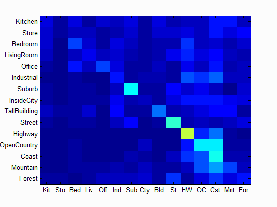
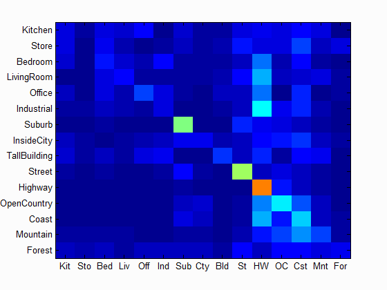
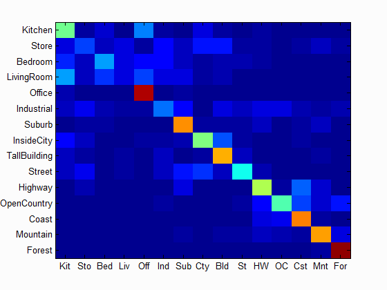
| Accuracy with tiny Image and 1 nearest neighbor classifier: 0.225 | Accuracy with tiny Image and K nearest neighbor classifier: K=11, Accuracy = 0.239 | Accuracy with bag of SIFT and K nearest neighbor classifier: K=11, Accuracy = 0.477 |
 |
 |
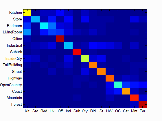 |
| Accuracy with bag of SIFT and linear SVM classifier: Num of Vocab = 10, Accuracy = 0.526 | Accuracy with bag of SIFT and linear SVM classifier: Num of Vocab = 20, Accuracy = 0.585 | Accuracy with bag of SIFT and linear SVM classifier: Num of Vocab = 50, Accuracy = 0.617 |
 |
 |
 |
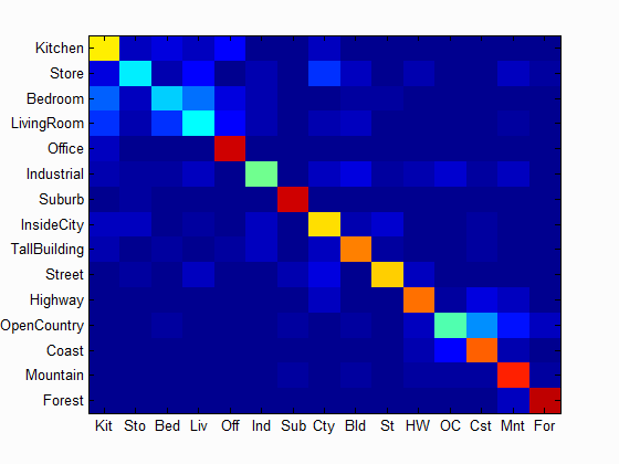
| Accuracy with bag of SIFT and linear SVM classifier: Num of Vocab = 100, Accuracy = 0.650 | Accuracy with bag of SIFT and linear SVM classifier: Num of Vocab = 200, Accuracy = 0.650 | Accuracy with bag of SIFT and linear SVM classifier: Num of Vocab = 400, Accuracy = 0.705 |
 |
||
| Accuracy with bag of SIFT and linear SVM classifier: Num of Vocab = 1000, Accuracy = 0.729 |
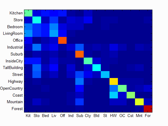
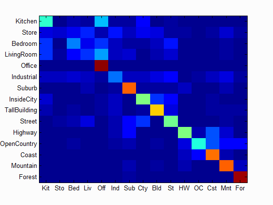
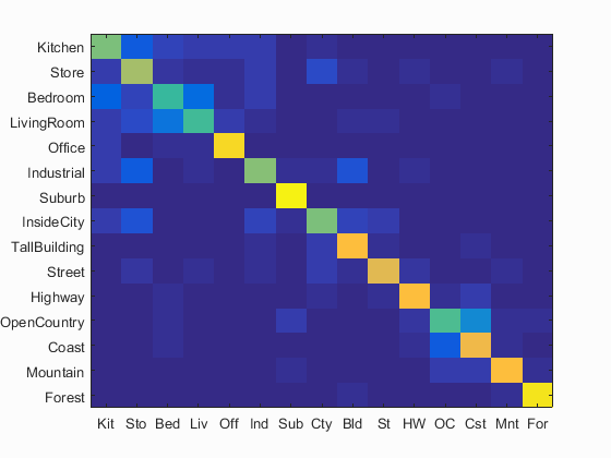
Scene classification results visualization
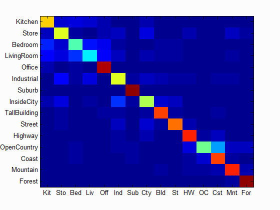
Accuracy (mean of diagonal of confusion matrix) is 0.729
| Category name | Accuracy | Sample training images | Sample true positives | False positives with true label | False negatives with wrong predicted label | ||||
|---|---|---|---|---|---|---|---|---|---|
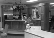
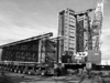
| Kitchen | 0.600 |  |
 |
 |
 |
 Industrial |
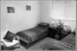
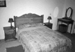
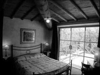
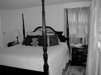
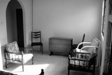
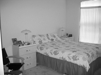 Bedroom |
 InsideCity |
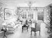
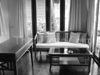
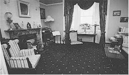
 LivingRoom |
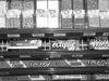
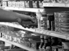
| Store | 0.660 |  |
 |
 |
 |
 LivingRoom |
 Industrial |
 InsideCity |
 Industrial |
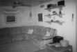
| Bedroom | 0.510 | 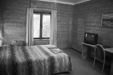 |
 |
 |
 |
 LivingRoom |
 InsideCity |
 Industrial |
 LivingRoom |
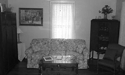
| LivingRoom | 0.520 | 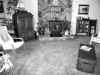 |
 |
 |
 |
 Industrial |
 Bedroom |
 Street |
 Office |
| Office | 0.910 | 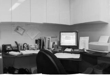 |
 |
 |
 |
 Kitchen |
 Store |
 Kitchen |
 LivingRoom |
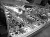
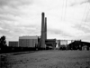
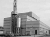
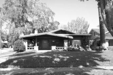
| Industrial | 0.610 |  |
 |
 |
 Street |
 Kitchen |
 InsideCity |
 TallBuilding |
|
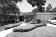
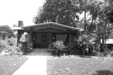
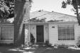
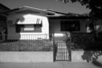
| Suburb | 0.970 | 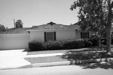 |
 |
 |
 |
 OpenCountry |
 OpenCountry |
 TallBuilding |
 LivingRoom |
| InsideCity | 0.600 |  |
 |
 |
 |
 TallBuilding |
 Store |
 Street |
 Store |
| TallBuilding | 0.830 |  |
 |
 |
 |
 InsideCity |
 Industrial |
 InsideCity |
 Bedroom |
| Street | 0.770 |  |
 |
 |
 |
LivingRoom |
 TallBuilding |
 InsideCity |
 Industrial |
| Highway | 0.830 |  |
 |
 |
 |
 OpenCountry |
 Street |
 Bedroom |
 OpenCountry |
| OpenCountry | 0.540 |  |
 |
 |
 |
 Bedroom |
 Mountain |
 Coast |
 Coast |
| Coast | 0.810 |  |
 |
 |
 |
 Highway |
 OpenCountry |
 OpenCountry |
 OpenCountry |
| Mountain | 0.840 |  |
 |
 |
 |
 Street |
 OpenCountry |
 Coast |
 Forest |
| Forest | 0.940 |  |
 |
 |
 |
 OpenCountry |
 Mountain |
 TallBuilding |
 Mountain |
| Category name | Accuracy | Sample training images | Sample true positives | False positives with true label | False negatives with wrong predicted label | ||||
Graduate Credit
I've test the performance with different vocabulary sizes, 10, 20, 50 100, 200, 400, 1000. The performance is listed below. Although size with 1000 has the highest accuracy, the calculating time is huge compared with others, 1000 vocabulary needs 3 hours to calculate while 400 needs 40 minutes and 200 needs about 18 minutes. And the accuracy is not improved that much. But the size of vocabulary has more effect on SVM classifier than KNN.
| Vocabulary Size | SVM Result | Nearest Neignbor result |
| 10 | 52.6% | 39.7% |
| 20 | 58.5% | 47.7% |
| 50 | 61.7% | 49.9 |
| 100 | 65.0% | 51.2% |
| 200 | 70.2% | 54.6% |
| 400 | 70.5% | 54.5% |
| 1000 | 72.9% | 51.8% |
I also do the cross validation. I chose the vocabulary with 400, and applied 1-vs-all linear svm classifier. Mix train images and test image together and randomly choose 100 images for training and another 100 for test. Then do such process 50 times and got the result: Mean = 46.96% and Std = 0.0516. The data is stored as name of "mean" and "std" in CV.mat. The code is proj_CV.m
I've also tried to test the performance on SUN dataset, and have already wrote the code. But my computer couldn't process such huge dataset. Therefore I could not give the result. The code is named as proj4_SUN.m, get_SUN_paths.m.
I also improved the knn classifier based on the paper from Boiman, Schechtman and Irani. . Let d1, . . . , dn be all the descriptors in the test image. The descriptor provided by training data is clustered based on the label and generated a cluster center NNC. And then for all descriptors d in test image, and all classes, do total=total+(di-NNC(di))^2. And assign the image to the class with lowest "total". The result is listed below.
 Accuracy = 55.6%