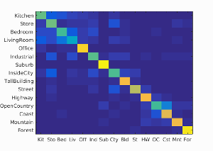
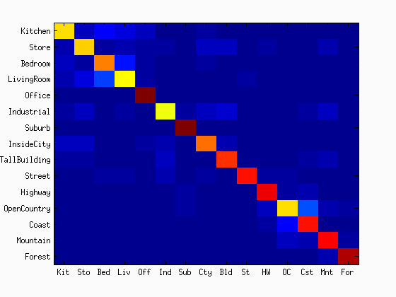
Example of a confusion matrix..

Tiny Image Features

One of the simplest way to convert an image to a comparable format is to use a tiny image feature. The idea is quite simple. We resize each of the train and test images to a very small one and use it as a feature vector. For example, if we resize an image to a 16 by 16 patch, we obtain a feature of 256 (16^2) dimensions. As we did for the SIFT features in Project 2, we normalize the features, which includes two procedures: making the feature zero-mean and forcing the norm to one. The code below generates the tiny image features:

% obtain tiny image features
patch_size = 16;
d = patch_size^2;
N = size(image_paths, 1);
image_feats = zeros(N, d);
image_feats_nonunit = image_feats;
image_feats_nonzeromean = image_feats;
for i = 1:N
    im = imread(image_paths{i});
    image_feats_tmp = imresize(im, [patch_size patch_size]);
    image_feats_nonzeromean(i, :) = reshape(image_feats_tmp, 1, d);
end
c = mean(mean(image_feats_nonzeromean(:, :)));
for i = 1:N
    image_feats_nonunit(i, :) = image_feats_nonzeromean(i, :) - c;
    image_feats(i, :) = image_feats_nonunit(i, :)./norm(image_feats_nonunit(i, :));
end

K Nearest Neighbors

Nearest neighbor method is a very simple method. Although it uses a lot of memories and can not beat state-of-the-art methods, it is still popular because of its straightforward implementation. When K=1, the classifier just computes the Euclidian distances of the test image with all the train images, and the one that has the minimum distance is selected as a correct model (predicted category). K-nearest neighbor method is just slightly more complicated than that. It stores the nearest neighbor one to the K nearest neighbor one, and the histgram is built based on the information. The category with the highest frequency is selected, so it may not necessarily be the one which has the smallest distance to the train image feature. The algorithm is implemented as follows:

% K nearest neighbors
D = vl_alldist2(train_image_feats', test_image_feats'); 
N = size(D, 2);
index = zeros(N, 1);
mode = 1; % 0: the nearest neighbor, 1: k-nn
predicted_categories = cell(N, 1);
if(mode == 0)     % only the nearest neighbor
    for i = 1:N
        [val, index(i, 1)] = min(D(:, i));
    end
    predicted_categories = train_labels(index);
elseif(mode == 1) % k nearest neighbor
    k = 30;
    for i = 1:N
        [val, ind] = sort(D(:, i));
        ind = ind(1:k);
        map = createMap();
        for j = 1:k
            map(cell2mat(train_labels(ind(j)))) = map(cell2mat(train_labels(ind(j)))) + 1;
        end
        key = keys(map);
        [hist_val, hist_ind] = sort(cell2mat(values(map)));
        predicted_categories{i, 1} = key{hist_ind(end)};
    end
end


function map = createMap()
    categories = {'Kitchen', 'Store', 'Bedroom', 'LivingRoom', 'Office', ...
       'Industrial', 'Suburb', 'InsideCity', 'TallBuilding', 'Street', ...
       'Highway', 'OpenCountry', 'Coast', 'Mountain', 'Forest'};
    value = zeros(1, size(categories, 2));
    map = containers.Map(categories, value);
end

The function createMap is used to build a histgram. In C++, this operation is as simple as the below, but it's a little trickier in Matlab because you cannot use a parameter before you initialize a corresponding key. There should be a better way than a map in Matlab.

% histgram in C++, 
map<string, int> m;
m[train_labels{i}]++;

Bag of Features

Although the tiny images are very simple and straightforward way to make a feature, but their accuracy is limited, and the features are lossy and not very informative. Another way to represent a image is to use bags of features. This is method is sometimes called bags of visual features, bags of sift features, etc. The original idea comes from the document classification. It classifies the documents based on how frequently specific words appear in a document. For example, if we frequently see the words such as "vector", "axis", "coordinate", and "parallel", that may be a math paper. In order to apply the bag of words model to computer vision, we first need to build the vocabulary like a "vector" and "axis". Our vocaburary is a sift feature. We represent a scene by building a histgram of these visual words. Therefore, a naive implementation of bag of features loses the spatial information such that which visual word is located where. We only see the distribution to classify a scene. The below code builds the visual words:

% build visual words
N = size(image_paths, 1);
sift_features = [];
for i = 1:N
    im = im2single(imread(image_paths{i}));
    step_size = 20;
    [locations, sift_features_per_image] = vl_dsift(im, 'step', step_size);
    sift_features = [sift_features, single(sift_features_per_image)];
end
[vocab, assignments] = vl_kmeans(sift_features, vocab_size);

We pull SIFT features from each of the train images and store all of them. These SIFT features need not to be samped finely because we don't need all the visual words to represent a scene. Those stored features are clustered by using k-means into k vocabraries, where k is the number of visual words. We build a histgram of these vocabraries for each of the train and test images. The exact same code is used to build the histgrams of the train and test images. The code is as follows:

% build histgrams of the visual words
load('vocab.mat')
vocab_size = size(vocab, 2); 
N = size(image_paths, 1);
step_size = 10;
image_feats = zeros(N, vocab_size);
for i = 1:N
    im = im2single(imread(image_paths{i}));
    [locations, sift_features_per_image] = vl_dsift(im, 'step', step_size);
    D = vl_alldist2(single(sift_features_per_image), vocab);
    map = zeros(1, vocab_size);
    for j = 1:size(D, 1)
        D_of_image = D(j, :);
        [val, ind] = min(D_of_image);
        map(1, ind(1, 1)) = map(1, ind(1, 1)) + 1;
    end
    map_zero_mean = map - mean(map);
    image_feats(i, :) = map_zero_mean ./ norm(map_zero_mean);
end

Support Vector Machine (SVM)

Support Vector Machine (SVM) is still used in many of the state-of-the-art machine learning and deep learning algorithms. Especially when the amount of train data is limited, SVM defeats most of the other classifiers such as the AdaBoost and random trees. The algorithm functions by projecting the train data set into a higher dimensional space and finds the linear separator that has the greatest margin to the data set. Since we have 15 categories to classify, we need to train 15 SVMs. We first create a label for each category, and plug the label and train features into 'vl_svmtrain'.

% train 15 SVN
for i = 1:num_categories
    labels = zeros(1, Ntrain);
    for j = 1:Ntrain
        if(strcmp(train_labels{j}, categories{i}))
            labels(1, j) = 1;
        else
            labels(1, j) = -1;
        end
    end
    [W(:, i) B(1, i)] = vl_svmtrain(train_image_feats', labels, LAMBDA);   
end

The output of the svmtrain is the weight vector W and offset B. Using these values, the fitness score of each test data can be computed as follows:

% compute the score and assign the category with the highest score
for j = 1:Ntest
    score = zeros(1, num_categories);
    xtest = test_image_feats(j, :)';%'
    max_score = -1e16;
    max_cat = [];
    for i = 1:num_categories
        score(1, i) = W(:, i)' * xtest + B(1, i);%'
        if(score(1, i) > max_score)
            max_score = score(1, i);
            max_cat = i;
        end
    end
    predicted_categories{j} = categories{max_cat};
end

Beyond Bags of Features

This section describes the implementation of the spatial pyramid and the pyramid match kernel. By adding the spatial information, the accuracy of the categorization was improved. The results are summarized in the following section.

Spatial Pyramid (Extra Credit)

In the spatial pyramid features, we extract the SIFT features at different resolutions. The level zero corresponds to the coarsest resolution of the image, and the algorithm repeatedly subdivide the image and computes the histgram of local features. This way, at a higher level, the resolutions of the image is finer, and the number of cells is increased. In this work, the design of the pyramid is the same as Lazebnik's; that is at 'l' level, we have 4^l bins. (Note that l starts with 0.) For the vocabulary size of M, we have dimensions of the vectors. (e.g. for M = 50 and L = 2, the dimension is 1050, for M = 400 and L = 3, the dimension is 34000.) At 'l' level, the original image is scaled by the factor of 1/(2^(L-l)). The following code is used to extract the spatial pyramid features.

% Build a spatial pyramid
for i = 1:N
    im = imread(image_paths{i});
    [original_H, original_W] = size(im);
    bin_count = 1;
    for j = 1:L+1 % current level + 1
        scale = 1.0/(2^(L-j+1));
        im_scaled = im2single(imresize(im, scale, 'bilinear'));

        [H, W] = size(im_scaled);
        [locations, sift_features_per_image] = vl_dsift(im_scaled, 'step', step_size);
        sift_feats = single(sift_features_per_image);
        h_lower = zeros(1, 2^(j-1));
        w_lower = zeros(1, 2^(j-1));
        h_upper = zeros(1, 2^(j-1));
        w_upper = zeros(1, 2^(j-1));
        for k = 1:2^(j-1)
            h_upper(1, k) = H/(2^(j-1)) * k;
            w_upper(1, k) = W/(2^(j-1)) * k;
            if(k > 1)
                h_lower(1, k) = h_upper(1, k-1);
                w_lower(1, k) = w_upper(1, k-1);
            end
        end
        
% For example, when L = 2
%                 h_lower = [ 0 1/4H 1/2H 3/4H ]
%                 w_lower = [ 0 1/4W 1/2W 3/4W ]
%                 h_upper = [ 1/4H 1/2H 3/4H H ]
%                 w_upper = [ 1/4W 1/2W 3/4W W ]
        for w = 1:size(w_upper, 2)
            for h = 1:size(h_upper, 2)
                ind_of_this_bin = find(locations(1, :) > w_lower(1, w)...
                                           & locations(2, :) > h_lower(1, h)...
                                           & locations(1, :) < w_upper(1, w)...
                                           & locations(2, :) < h_upper(1, h));
                feats_of_this_bin = sift_feats(:, ind_of_this_bin);
                D = vl_alldist2(feats_of_this_bin, vocab);
                map = zeros(1, M);
                for l = 1:size(D, 1)
                    D_of_image = D(l, :);
                    [val, ind] = min(D_of_image);
                    map(1, ind(1, 1)) = map(1, ind(1, 1)) + 1;
                end
                map_zero_mean = map - mean(map);
                image_feats(i, bin_count, :) = map_zero_mean ./ norm(map_zero_mean);
                bin_count = bin_count + 1;
            end
        end
    end
end

Pyramid Match Kernel (Extra Credit)

Pyramid match kernel is very intuitive method. Since the higher level of features are extracted from the finer resolutions, we weigh the features of the higher level more than the ones from a lower level. The weights are inversely proportional to the 'distance', which means that the features at 'l' level is weighted by 1/(2^(L-l)). (Remember that the image at 'l' level is scaled by a factor of 1/(2^(L-l)).) Since the number of matches found at level 'l' also includes all the matches found at the finer level 'l+1', the entire pyramid match kernel can be expressed as follows: The best study material to under stand this concept is Lazebnik's slides. The below figure summarizes the concept.

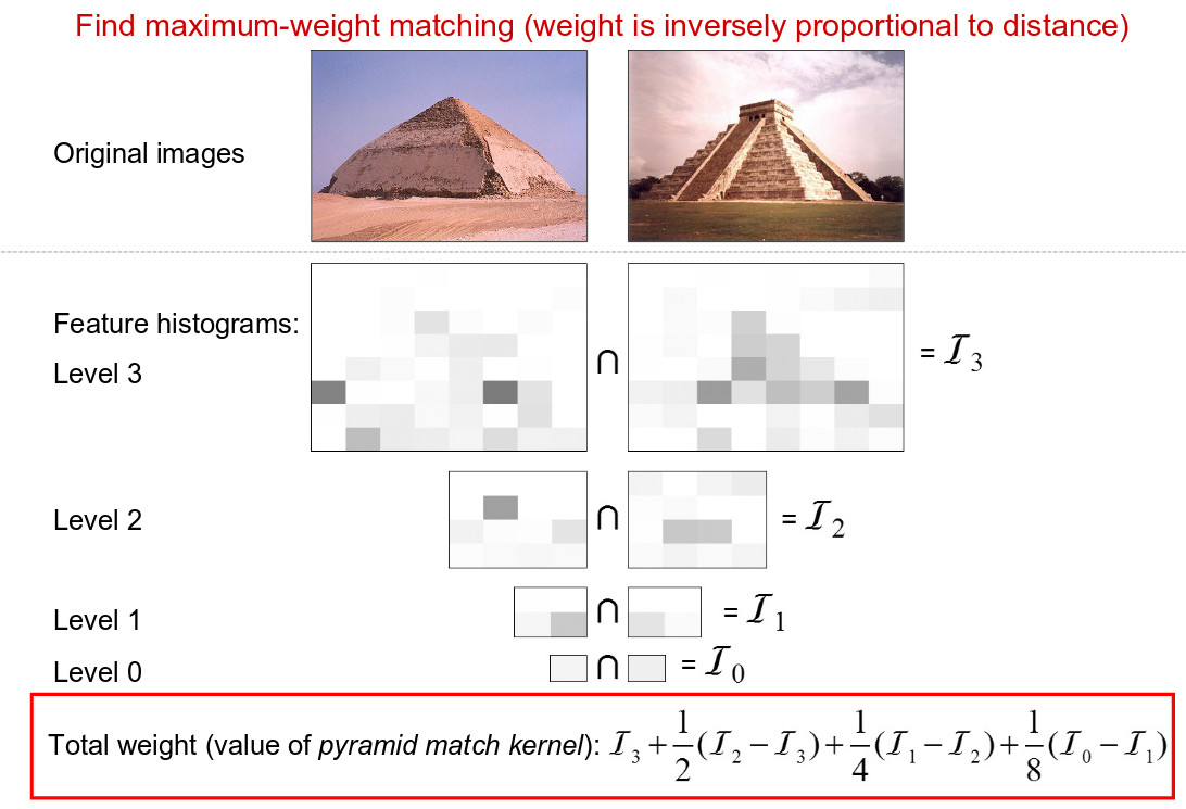
The Lazebnik's slide to explain the pyramid match kernel

The results of the spatial pyramid are discussed in the following section. The code below is used for this experiment.

% pyramid match kernel
weighted_train_image_feats = zeros(Ntrain, (4^(pyramid_level + 1)-1)/3, d);
for i = 1:Ntrain
    weighted_train_image_feats(i, 1, :) = (1.0/2^(pyramid_level)) * train_image_feats(i, 1, :);
    l = 1;
    n_of_this_bin = 0;
    for j = 2:size(train_image_feats, 2)
        weight = 1.0/(2^(pyramid_level - l + 1));
        weighted_train_image_feats(i, j, :) = weight * train_image_feats(i, j, :);
        n_of_this_bin = n_of_this_bin + 1;
        if(n_of_this_bin >= 4^l)
            l = l + 1;
            n_of_this_bin = 0;
        end
    end
end
concatenated_train_feats = reshape(weighted_train_image_feats, [Ntrain,  dim_of_concat]);
for i = 1:num_categories
    labels = zeros(1, Ntrain);
    for j = 1:Ntrain
        if(strcmp(train_labels{j}, categories{i}))
            labels(1, j) = 1;
        else
            labels(1, j) = -1;
        end
    end
    [W(:, i) B(1, i)] = vl_svmtrain(concatenated_train_feats', labels, LAMBDA); 
end
weighted_test_image_feats = zeros(Ntest, (4^(pyramid_level + 1)-1)/3, d);
for i = 1:Ntest
    weighted_test_image_feats(i, 1, :) = (1.0/2^(pyramid_level)) * test_image_feats(i, 1, :);
    l = 1;
    n_of_this_bin = 0;
    for j = 2:size(test_image_feats, 2)
        weight = 1.0/(2^(pyramid_level - l + 1));
        weighted_test_image_feats(i, j, :) = weight * test_image_feats(i, j, :);
        n_of_this_bin = n_of_this_bin + 1;
        if(n_of_this_bin >= 4^l)
            l = l + 1;
            n_of_this_bin = 0;
        end
    end
end
concatenated_test_feats = reshape(weighted_test_image_feats, [Ntrain, dim_of_concat]);

% and use the method described in the svm section

Results

This section reports the results of the several experiments.

Results of the submitted codes

The default codes need to satisfy the following criteria:

1. The pipeline (without) vocabulary building runs in 10 mins total for any of the three conditions below
2. Tiny images representation and nearest neighbor classifier (min accuracy 15%)
3. Bag of SIFT representation and nearest neighbor classifier (min accuracy 45%)
4. Bag of SIFT representation and linear SVM classifier (min accuracy 55%)

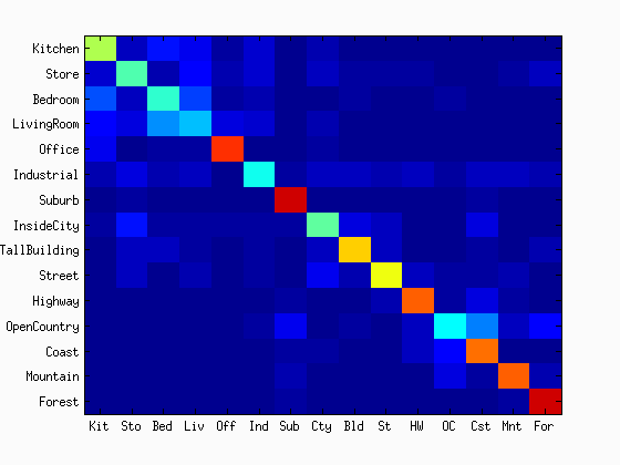
The submitted code of the author achieves the following performance:

	Tiny Image + KNN	BoVW + KNN	BoVW + SVM
Time[s]	14.67	520.78	492.16
Accuracy[%]	23.5	50.2	61.7

In the default settings, the KNN method uses K = 5. The size of the vocaburalies is 50, and the step size for the sift feature extration is 4. The vocabularies are build by SIFT features with the step size of 20. The SVM uses the lambda of 0.0001. The experiments are conducted with MATLAB2016a on Ubuntu 14.04 64-bit. The processor is Intel Core i7-3770 CPU @ 3.40GHz x 8, and available memory size is 4GiB. The default setting does not use the spatial pyramid.

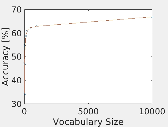
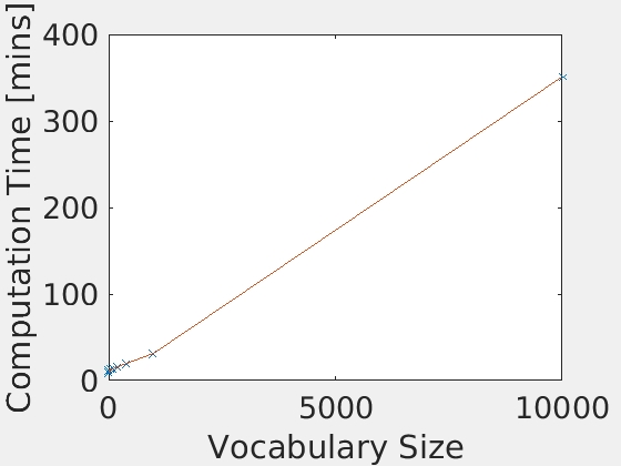
Effect of the Vocabulary Size (Extra Credits)

The author ran the Bag of SIFT with the SVM classifier with various vocabulary sizes. Throughout the experiments, the other free parameters than the vocabulary size such as the lambda, the step sizes, and the SIFT feature dimension are fixed. The sizes of the vocabulary tested in this experiments are 10, 20, 50, 100, 200, 400, 1000, and 10000. The below figures summarizes the accuracies and the computational time with many different vocabulary sizes.

Accuracy vs vocab sizes	Time elapsed vs vocab size

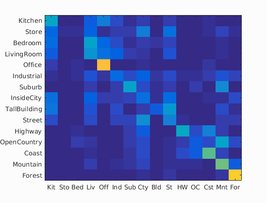
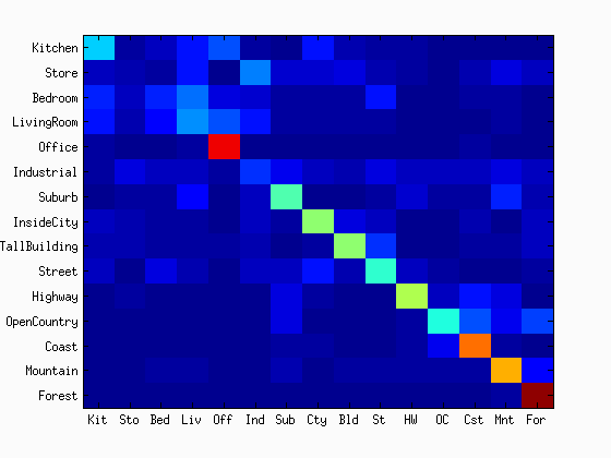
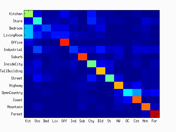
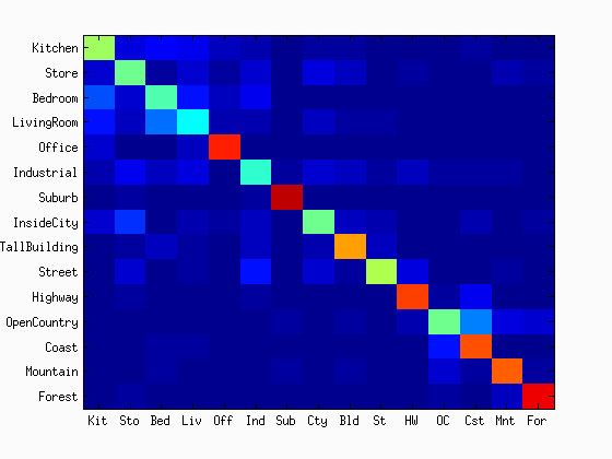
As shown in the figures, the accuracy was increased as the increase in the vocabulary size. Although the accuracy was monotonically increased with the tested range of the vocabulary sizes, we did not see as much improvement after 400. The computational time was almost linearly increased with the increase in the vocaburary size. From these results, the vocabulary size of 400 to 1000 may be a good selection considering both the accuracy and computational time. The reason why it did not work very well with a lower number of vocabulary sizes would be explained with the below figures. They are the confusion matrices with the different sizes of the vocabulary sizes. At a low number of vocabularies, the performance of one category is much better than the others. Sometimes, the chosen visual words are good enough to represent a certain category, but the same does not apply for others.

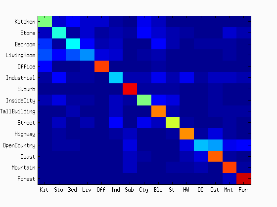vocab = 10	vocab = 20	vocab = 50	vocab = 100
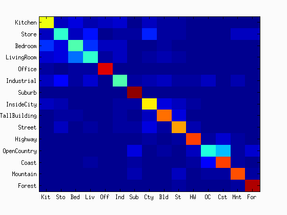vocab = 200	vocab = 400	vocab = 1000	vocab = 10000

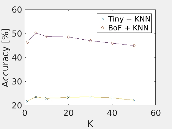
Results with many different Ks

The author tested the performance of the K-nearest neighbors method with tiny image features and bags of SIFT. The choice of K for the default setting is the one that maximized both of the features. The below figure and table summarize the results.

	K=1	K=5	K=10	K=20	K=30	K=40	K=50
TinyImage	21.7	23.5	22.9	23.4	23.5	23.1	22.1
BoVW	46.3	50.2	48.8	48.5	47.0	45.9	44.9

Accuracy with various Ks

Results of the spatial pyramid

You can use the spatial pyramid by setting the parameters below:

use_spatial_pyramid = 1;
pyramid_level = 2; % L is zero-based. L=0->1, L=1->5, L=2->21, L=3->85...

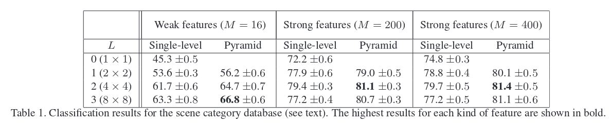
These switches live in proj4.m. First, the author compares the results of the spatial pyramid with the ones without spatial pyramid for three different vocab sizes (M). The below table summarizes the resutls:

Accuracies with or without spatial pyramid
	M = 50	M=200	M = 400
Spatial Pyramid	68.1%	75.8%	77.5%
No Spatial Pyramid	61.7%	66.9%	68.1%

In this experiment, lambda = 0.0001, the step size to build codebook and to extract sift features were 20 and 4, respectively. The maximum level of the pyramid was L=2, which means that the total number of bins were 1 + 4 + 16 = 21. In all of the vocab sizes, the spatial pyramid improved the accuracy. In order to explore the effect of the pyramid level, another experiment was done with 4 different Ls. The below summarizes the results:

Accuracies with different pyramid levels
L = 0	L = 1	L = 2	L = 3
61.7%	69.9%	68.1%	70.7

All the parameters are default settings except 'use_spatial_pyramid' and 'pyramid_lvel'. You should be able to replicate these results by turning on the spatial pyramid and changing the pyramid level. One may think that the higher pyramid level results in the better results, but this is not always the case. In fact, the Lazebnik's conducted the same experiments, and the higher level of pyramid did not necessarily achieve the highest accuracy.

Lazebnik's results

Results of the best Bags of SIFT features and SVM

The below is the results that achieved the maximum accuracy. The step size is 2, the pyramid level L = 2, lambda = 0.00001, and the vocabulary size is 400. It took more than 3 hours on the i7 desktop machine. It achieved 78.9% of accuracy. Although the accuracy is lower than the Lazebnik's results, the spatial pyramid dramatically improved the overall performance. The workspace variables are saved to best_result.mat. You can quickly see the results by loading this mat file. Download it from here: https://www.dropbox.com/s/bci5k4m8pqswh4i/best_result.mat?dl=0 (192MB)

Scene classification results visualization

Accuracy (mean of diagonal of confusion matrix) is 0.789

Category name	Accuracy	Sample training images		Sample true positives		False positives with true label		False negatives with wrong predicted label
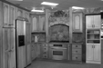
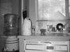
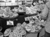
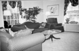
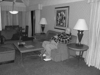
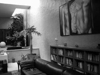
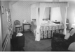
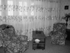
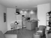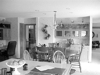
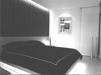
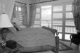
Kitchen	0.650					LivingRoom	InsideCity	Bedroom	InsideCity
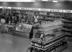
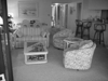
Store	0.660					InsideCity	LivingRoom	Kitchen	Office
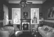
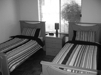
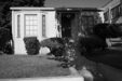
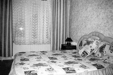
Bedroom	0.740		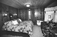			LivingRoom	Street	Office	LivingRoom
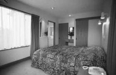
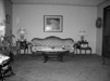
LivingRoom	0.610		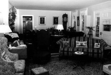			Bedroom	Bedroom	Store	Bedroom
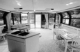
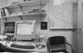
Office	0.990		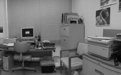			Kitchen	Bedroom	Kitchen
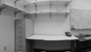
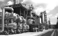
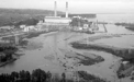
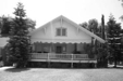
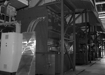
Industrial	0.600					InsideCity	Street	Office	Coast
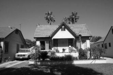
Suburb	0.990		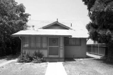			InsideCity	Industrial	LivingRoom
InsideCity	0.750					Store	Bedroom	OpenCountry	Kitchen
TallBuilding	0.820					Industrial	Store	Mountain	Industrial
Street	0.850					LivingRoom	Bedroom	LivingRoom	Bedroom
Highway	0.880					Store	Store	Mountain	Suburb
OpenCountry	0.650					Coast	Coast	Forest	Coast
Coast	0.850					TallBuilding	OpenCountry	OpenCountry	OpenCountry
Mountain	0.860					Highway	Industrial	OpenCountry	OpenCountry
Forest	0.940					Mountain	Mountain	Suburb	OpenCountry
Category name	Accuracy	Sample training images		Sample true positives		False positives with true label		False negatives with wrong predicted label