Project 4 : Scene Recognition with Bag of Words
Bag of Words Model.
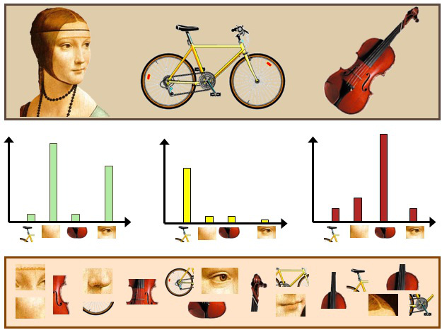
The goal of this project is to implement scene recognition using the concept of bag of features. The idea has been derived from the concept of bag of textures which is a popular and accurate technique used in natural language processing for classification of text into different category. In this model, a text (such as a sentence or a document) is represented as the bag (multiset) of its words, disregarding grammar and even word order but keeping multiplicity. In document classification, a bag of words is a sparse vector of occurrence counts of words; that is, a sparse histogram over the vocabulary. In computer vision, a bag of visual words is a vector of occurrence counts of a vocabulary of local image features. We use three ways of representing our images using appropriate features
- Tiny images.
- Bag of sift. It can be further used alongwith one of the following:
- Spatial pyramid
- Soft assignment i.e Kernel codebook encoding
- Fisher vector encoding.
- Nearest Neighbor
- Naive Bayes Nearest Neighbor (NBNN)
- Support Vector Machine
We will look at each step and its implementation individually. An effort to compare accuracy using all of the above mentioned steps and their combination has been made.
Tiny image Representation
The "tiny image" feature, inspired by the work of the same name by Torralba, Fergus, and Freeman, is one of the simplest possible image representations. One simply resizes each image to a small, fixed resolution (we recommend 16x16). It works slightly better if the tiny image is made to have zero mean and unit length. This is not a particularly good representation, because it discards all of the high frequency image content and is not especially invariant to spatial or brightness shifts. The complexity of classification task is greatly reduced using tiny images though the accuracy obtained is very low. After having represented images as tiny images, the classification task for done using following two independent techniques:
- Nearest Neighbor: For classification of tiny images using nearest neighbor, the best results are obtained with k =11. The accuracy of 24.2% was obtained for our data set. Here the results obtained are as shown below.
- Support Vector Machine: On using the support vector machine for image classification, the accuracy of about 18% is obtained. The linear classifiers will have a lot of trouble trying to separate the classes and may be unstable
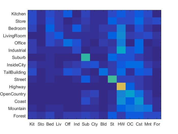
Accuracy (mean of diagonal of confusion matrix) is 0.242
Bag of SIFT features
We use SIFT features to represent images in feature space. But before we can represent our images as bag of feature histograms, we build a vocabulary of visual words. We form this vocabulary by sampling a huge number of local features from our training set and then cluster them with kmeans algorithm. The number of kmeans clusters is the size of our vocabulary and the size of our features. For example, you might start by clustering many SIFT descriptors into k=50 clusters. This partitions the continuous, 128 dimensional SIFT feature space into 50 regions. For any new SIFT feature we observe, we can figure out which region it belongs to as long as we save the centroids of our original clusters. Those centroids are our visual word vocabulary. Now, SIFT features are extracted from all the images in training set. These are then mapped to one of the clusters in the vocbulary. A normalised histogram is then built for all the images in training set. This set forms the training_feature_set. Now, the exact procedure is repeated for the testing set forming testing_feature_set. The normalized histogram is now the feature representation.
- Nearest Neighbor: The features for all the images are compared with all the training_feature_set. The nearest neighbor is obtained for all the images and the label of nearest neighbor is assigned to the test image. We can use k-NN or 1-NN. Both of have been implemented for testing accuracy. The accuracy of about 48.2% is obtained for the vocabulary size of 500 and with the SIFT size = 5 and step = 10.
- Naive Bayes Nearest Neighbor (NBNN): This algorithm is better than the standard nearest neighbor method. Instead of calculating the distance between a test image and an individual image and assigning the label of one with least distance, we calculate the distance of test image with all the images from a particular class and calculate the sum of all the distances. The class with minimum distance is then assigned to the test image. It has proven to be more accurate as compared to k-nearest neighbor method.
- Support Vector Machine: Here we take the features from one class and mark then as positive labels and images from all other classes and mark then as negative labels. Using SVM, the feature space is partitioned by a learned hyperplane and test cases are categorized based on which side of that hyperplane they fall on. Despite this model being far less expressive than the nearest neighbor classifier, it will often perform better. The prediction from a nearest neighbor classifier will still be heavily influenced by frequent visual words, whereas a linear classifier can learn that those dimensions of the feature vector are less relevant and thus downweight them when making a decision. This procedure is repeated for all the classes and we have fifteen 1-vs-all SVM classifiers. The accuracy of 65.6% was obtained for the classification task using SVM. The vocabulary size of 500 was used.
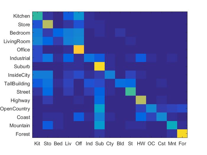
Accuracy (mean of diagonal of confusion matrix) is 0.482

Accuracy (mean of diagonal of confusion matrix) is 0.613

Accuracy (mean of diagonal of confusion matrix) is 0.656
Adding Spatial information to the feature space
The bag of SIFT features is quantised and thus loses the spatial information. Adding spatial information to the features, improves the data representation and thus results in better accuracy. Spatial information was added to the features by implementing the spatial pyramid feature representation described in Lazebnik et al 2006. For level 0, the entire image is considered a block and bag of features for it is added to features. For level 1, the image is divided into 4 halves and the bag of features for each block as added as feature for that image. For level 2, we divide the image into 16 blocks and bag 0f features for each is added to the features of that image.
Accuracy (mean of diagonal of confusion matrix) is 0.464
Soft Assignment i.e Kernel Codebook encoding
While computing the bag of features, we take the individual feature in the image, compare it with the vocabulary centers i.e cluster center and assign the image feature to the center with least distance. In 'Soft Assignment' instead of assigning the entire weight of that feature to one cluster, we look at its k nearest neighbors and assign them weight which is proportional to the distance from the centre. The lesser the distance, more will that feature contribute for that particular cluster. This has been implemented and the accuracy was found out to be
Accuracy (mean of diagonal of confusion matrix) is 0.613
Fisher vector encoding
Instead of using SIFT feature, if we use Fisher Vector encoding for feature representation the accuracy is very high. The fisher vector encoding technique has been implemented and the accuracy found using this is very high i.e 77.4% The support vector machine classifier was used for classification
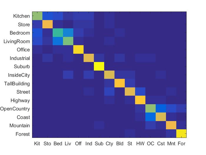
Accuracy (mean of diagonal of confusion matrix) is 0.774
Function for implementation of fisher vector encoding
%example code
function [ m,c,p] = fisher_encoding( image_paths, vocab_size )
vocab_features = [];
for i=1:1:size(image_paths,1)
    filename = strjoin(image_paths(i));
    im = imread(filename);
    im=single(im);
    [locations features] = vl_dsift(im,'step',10,'fast');
    features = single(features);
    vocab_features = [vocab_features features];
end
[mean,covariance,priors]=vl_gmm(vocab_features, vocab_size);
end
Various testing performance:
1) Experiments with different vocabulary size:
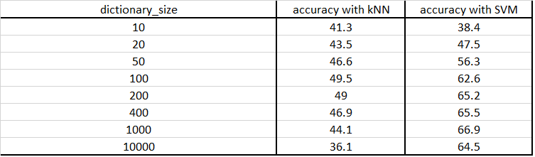
The size of SIFT feature was fixed to 10 and the step was set to 5 and the vocabulary was built with different number of cluster sizes. This dictionary was then used to compute classification task and the accuracy was noted. Results are as below:

|
It can be clearly seen that the accuracy goes up as the size of vocabulary increases till size is 1000. We checked at size =10000, and the accuracy dropped as can be seen in the table. It has not been plotted to maintain the scale of graph.
2) Effect of different 'k' in knn on accuracy of tiny images:
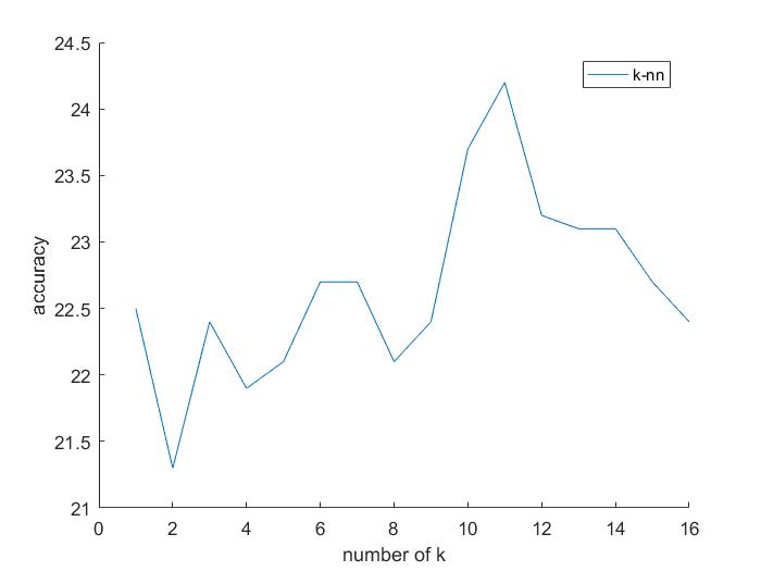
Accuracy (mean of diagonal of confusion matrix) is 0.242 for k=11
| Category name | Accuracy | Sample training images | Sample true positives | False positives with true label | False negatives with wrong predicted label | ||||
|---|---|---|---|---|---|---|---|---|---|
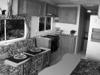
| Kitchen | 0.610 | 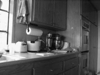 |
 |
 |
 |
 Bedroom |
 Office |
 Office |
 Industrial |
| Store | 0.510 |  |
 |
 |
 |
 LivingRoom |
 Street |
 Highway |
 Suburb |
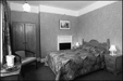
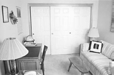
| Bedroom | 0.460 |  |
 |
 |
 |
 Highway |
 LivingRoom |
 Street |
 Kitchen |
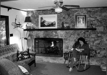
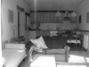
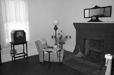
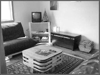
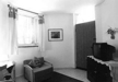
| LivingRoom | 0.270 | 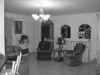 |
 |
 |
 |
 Industrial |
 Store |
 Bedroom |
 Kitchen |
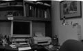
| Office | 0.820 |  |
 |
 |
 |
 Bedroom |
 Kitchen |
 Kitchen |
 Kitchen |
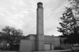
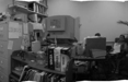
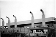
| Industrial | 0.450 |  |
 |
 |
 |
 Kitchen |
 Street |
 TallBuilding |
 Coast |
| Suburb | 0.970 |  |
 |
 |
 |
 Store |
 Mountain |
 OpenCountry |
 Street |
| InsideCity | 0.490 |  |
 |
 |
 |
 Street |
 Kitchen |
 Industrial |
 Coast |
| TallBuilding | 0.830 |  |
 |
 |
 |
 Mountain |
 Street |
 Forest |
 Industrial |
| Street | 0.670 |  |
 |
 |
 |
Bedroom |
 Forest |
 InsideCity |
 InsideCity |
| Highway | 0.780 |  |
 |
 |
 |
Store |
 OpenCountry |
 Coast |
 Suburb |
| OpenCountry | 0.460 |  |
 |
 |
 |
Suburb |
 InsideCity |
 Highway |
 Coast |
| Coast | 0.800 |  |
 |
 |
 |
 OpenCountry |
 OpenCountry |
 OpenCountry |
 OpenCountry |
| Mountain | 0.790 |  |
 |
 |
 |
 Industrial |
 LivingRoom |
 Office |
 Suburb |
| Forest | 0.930 |  |
 |
 |
 |
 OpenCountry |
 OpenCountry |
 Mountain |
 Mountain |
| Category name | Accuracy | Sample training images | Sample true positives | False positives with true label | False negatives with wrong predicted label | ||||