Project 4 / Scene Recognition with Bag of Words
Introduction
This goal of this assignment was to explore scene recognition through the scope of the bag of words model. The bag of words model is one in which images are described by a histogram containing the frequency of visual words. By comparing the histograms of testing images and labeled training images, one can determine the most likely label of the testing images.
Specifically, this assignment asks us to classify images into 1 of 15 scene categories (labels). This 15 scene dataset was originally introduced in Lazebnik et al. 2006. To perform the classification, we try 3 distinct strategies:
1. Tiny Image Features with Nearest Neighbor Classifier
2. Bag of Words Feature Representation (SIFT) with Nearest Neighbor Classifier
3. Bag of Words Feature Representation (SIFT) with Linear SVM Classifier
This report will proceed as follows: I will sequentially describe the methodology and show the results for the above 3 strategies for scene recognition. I will then have a section in which I describe and show the results for the various bells & whistles additions I completed (Vocab Size Consideration, Spatial Pyramid, GIST, Kernel Codebook Encoding, RBF SVM Kernel).
Tiny Image Features with Nearest Neighbor Classifier
Methodology
1. For both the training images and the testing images, crop out a 'central square' from the original image so that the image is now 'square' (i.e. get rid of as few outer rows/columns as possible)
2. Resize the resultant square image to 16x16 pixels. Reshape this matrix of pixels to 1x256, and make this vector zero mean and unit length. This vector is now the 'tiny image feature' for this image.
3. Take the pairwise distance between each test image tiny feature and all of the training images tiny features. The label of the training feature that is the smallest distance away from any given test feature is assigned as the scene classification for that test image. This is effectively the methodology for the 1-nearest neighbor classifier.
Results
 (Accuracy: 22.60%, Runtime: 14 Seconds, No Explicit Parameters Given)
At first glance, an accuracy of 22.60% might seem terrible. It's important to recognize though that if one just guessed randomly you would get an accuracy of ~7% (1/15 since there are 15 categories). Thus, this very simple Tiny Image Feature together with the Nearest Neighbor Classifier is very fast and is more than 3 times better than guessing.
Bag of Words Feature Representation (SIFT) with Nearest Neighbor Classifier
Methodology
1. Generate SIFT features from every training image, and append each 128 x d (where d is the number of SIFT features returned for a given image) matrix together.
2. Use the above matrix to generate the 'bag of words'. Essentially run k-means on the above matrix where k is the desired vocab size (I use 200). The resultant 128 x k cluster centers are the visual words we will use to generate histograms.
3. Generate SIFT features again for both the training and testing images. For each image's feature representation, take the distance between each of its SIFT features and all of the visual words that were calculated in the previous step. The shortest distance visual word to each image SIFT feature is the word that we will assign.
4. Create a histogram of the counts of visual words for each training/testing image based on the output of the previous step. This normalized histogram (normalized to ensure that larger versions of the same image don't have higher vocabulary counts) is now the 'bag of words representation' of the image.
5. Take the pairwise distance between each test image bag of words histogram and all of the training images' bag of words histograms. The label of the training histogram that is the smallest distance away from any given test histogram is assigned as the scene classification for that test image (note: 1-nearest neighbor, exactly the same as the tiny images nearest neighbor methodology from the section above)
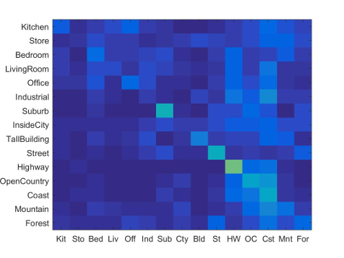
Results
 (Accuracy: 51.60%, Runtime: 3:07 Minutes, SIFT_Size: 6. SIFT_Step: 10., Vocab Size: 200)
Clearly, this bag of sift words implementation produces much better results than the tiny image features implementation. It's worth pointing out that for my nearest neighbor classifier implementation, I'm still using 1-NN (just as I did for the Tiny Image Feature strategy). It's likely that if I were to consider more neighbors (i.e. potentially 5 nearest neighbors), and have each of those nearest 5 matches 'vote' towards the final label, I would get a higher accuracy. Additionally, I'd like to note here that in my original implementation, I used a vocab size of 300, which yielded an accuracy of ~54%, but also took ~4:15 minutes (longer than the alotted time).
Bag of Words Feature Representation (SIFT) with Linear SVM Classifier
Methodology
1. Generate a visual vocabulary using the same methodology described in the previous section (create SIFT features for all training images, use k-means (k = 200))
2. Generate bag of words histogram representations for each image using the same methodology described in the previous section (generate SIFT features for training and testing images, take distance between all SIFT features and all possible visual words, create histogram of the number of times a given visual word is assigned to a feature in the image)
3. Train 15 1 v. all linear SVMs on the training histograms (one for each scene). This effectively amounts to fitting a hyperplane that tries to best separate the histogram vectors corresponding to a given scene and all of the other histograms vectors. Store the resulting weight vector and offset term for each of the 15 runs.
4. For each of the 15 scenes, calculate the resulting 'score' for each test image (where w is the 200x1 weight vector, X is the 200x1500 test image feature matrix, and b is the offset scalar):

The model that results in the most positive score for a given test image is now the classification given to that image (i.e. if a test image scores the most positive score on the kitchen v. all model, its classification is kitchen)
Results
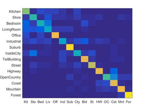 (Accuracy: 65.30%, Runtime: 3:13 Minutes, SIFT_Size: 6. SIFT_Step: 10., Vocab Size: 200, Lambda: 0.0001)
(Accuracy: 65.30%, Runtime: 3:13 Minutes, SIFT_Size: 6. SIFT_Step: 10., Vocab Size: 200, Lambda: 0.0001)
Of all the three strategies, this one seems to perform the best. Note that the image representation (Bag of Sift Words) is the same for both this strategy and the Bag of Sift Words with Nearest Neighbor Classifier strategy. And yet, this strategy yields ~14% better accuracy. This ~14% difference can be attributed to the use of the Linear SVM Classifier rather than the Nearest Neighbor Classifier. The results here should not be interpreted as saying that Linear SVM should always be preferred to Nearest Neighbor; recall from the previous section that I was just using 1-NN. It is possible that if I were to increase the number of nearest neighbors I consider, I could get a final accuracy similar/better to the one I have here.
Bells & Whistles Work
Once I had the initial 3 strategy implementations completed, I decided to add on bells and whistles work to the best performing one (Bag of Words with Linear SVM) to try to get a higher accuracy score.
Vocabulary Size Consideration
The first thing I did was to test the relationship between vocabulary size and accuracy. Note that the results shown in the section above for Bag of Words with Linear SVM are gotten by using a vocabulary size of 200. Thus I was curious to see if changing this vocabulary size could yield meaningfully diffent results:
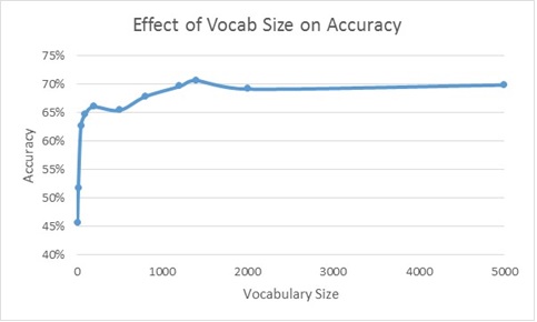
Clearly, it appears as though accuracy increases fairly monotonically with vocabulary size. Admittedly, there are some dips in accuracy that occur at a vocab size of 500 and 2000, but I'm willing to say that's probably an artifact of a 'bad' k-means run (to create the vocabulary). Additionally, it's worth noting that it looks like there are diminishing returns to increasing vocabulary size - Accuracy precipitously increases as you increase vocabulary size from 10 to 100 (46% to 65%), but from here the accuracy increase from 100 to 5000 is relatively small (65% to 70%).
Having said all that, to generate the highest accuracy rate, this plot suggests that
I should use a vocabulary size of 5000. What's not shown on the plot, however, is computation
time. My code took over an hour to create the results for a vocabulary size of 5000.
Thus, in an attempt to balance computation time and accuracy, I increase the vocabulary size
of the Bag of Words Feature Representation (SIFT) with Linear SVM Classifier implementation
from 200 to 600. The results of this increase in vocabulary size are shown below:
 (Accuracy: 66.20%. Vocab Size: 600. SIFT_Size: 6. SIFT_Step: 10. Lambda: 0.0001.)
Note - this result will serve as the 'baseline' that I will add additional Bells & Whistles items to in the next section.
Additional Bells & Whistles Work
In this section, I will briefly describe the intuition/methodologies behind each of the additional Bells & Whistles items I completed. I will then present the results gained by including these items to my 'baseline' implementation shown in the previous section. Note that when I show the results of including each Bells & Whistles item, I show the 'marginal impact of inclusion' i.e. the accuracy that resulted by including only one Bells & Whistles item at a time with the baseline implementation. I think looking at the results in this way is instructive since it avoids the consideration of the order in which items were piled on top of each other (i.e. potential cross terms)
Spatial Pyramid
This Bells & Whistles item attempts to address the fact that the traditional bag of words model is devoid of any spatial information. The histogram feature that is kept for the image contains the counts for a given visual word, but it doesn't contain any information related to where that word was found in the image.
The Spatial Pyramid attempts to overcome this by creating histograms for subsections of the image, and appending these histograms to the original bag of words histogram. By doing this, one not only knows how often a given word was present, but they also have some sense of where the word was located.
My implementation of the Spatial Pyramid roughly follows that of Lazebnik et al 2006. In particular, I have one histogram for the whole image (Level 0). Then I split the image into 4 quadrants (Level 1) and create/append one histogram from each quadrant to the histogram from Level 0. I then split each quadrant into 4 more quadrants (Level 2) and create/append 16 more histograms to the existing histogram vector.
Note that when I append each level's histograms to the final histogram vector, I follow the suggestion of Lazebnik to weight each level's histogram differently. Intuitively, this makes sense as we want to weight the histograms from finer pyramid levels more. The weights I use are as follows:
Kernel Codebook Encoding
Kernel Codebook Encoding is effectively a method that allows for 'soft assignment' of visual words to histogram bins. Recall from earlier sections that normally with bag of words, we take the distance between each SIFT feature in an image and the words in the visual vocabulary. The word that is the nearest distance from a given SIFT feature gets incremented in the histogram. Using Kernel Codebook Encoding, not only the nearest distance word, but instead the N nearest words will get incremented in the histogram for the image (I use an N of 3).
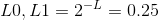
In terms of what value to increment each of the 3 nearest histogram word places by, I use the following scheme (where d is distance, and sigma is 10^12):

This weighting scheme is in the spirit of Philbin et al 2008 (they use -d^2 instead of -d^5). The scheme ensures that the nearest distance gets the highest increment value, and the other two distances get smaller increment values. By using an exponent of 5 rather than 2, I essentially penalize further distances more.
GIST
The GIST descriptor is similar to the SIFT descriptor, but is applied to an entire image rather than to a keypoint. Essentially, this descriptor applies oriented Gabor filters over different scales and averages the filter 'energy' in each bin. With 8 orientations, 4 scales, and 16 bins, the GIST descriptor is 512 dimensions for an entire image.
My implementation leverages the LMgist code from Oliva and Torralba. My code simply calculates the GIST descriptor for each image and appends this 512 dimensional vector to the existing bag of words histogram.
RBF SVM Kernel
In the Bag of Words Feature Representation (SIFT) with Linear SVM Classifier section, I used a Linear SVM Classifier. Essentially this means that a hyperplane is trying to draw the separation for the one v. all (in R2 the hyperplane can be though of as a line). The RBF SVM Kernel allows us to use a surface rather than a hyperplane to determine separations for one v. all. In particular, using the RBF kernel is akin to having a separating surface that is based on a combination of bell-shaped surfaces that are centered at each support vector.
The RBF kernel can be calculated as follows (I use a sigma of 0.35):
To use this RBF kernel instead of the linear SVM, I first calculate the RBF kernel where both x and y are training features. I then use this kernel to train 15 one v. all SVMs. To then make predictions, I calculate another RBF kernel where x is the test features and y is the train features. For each model I use this new RBF kernel to come up with a score (similar to linear SVM); the label corresponding to the most positive score for a given test image is the label assigned as the predicted classification.
Results
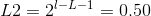
Clearly, the marginal impact of inclusion for the Spatial Pyramid, the Kernel Codebook Encoding, and GIST are positive. We see that because accuracy increases from the Baseline of 66% to 70%, 72%, and 76%, respectively. Regrettably, the inclusion of RBF has a negative marginal impact of inclusion, as accuracy goes down from 66% to 58%.
I don't think that it is right to conclude from the results above that RBF unequivocally is bad for performance on this 15-scene dataset. I say that because the accuracy of this result is highly sensitive to the sigma parameter (kernel width) in the RBF kernel generation process. From what I observed just from manual tuning, it didn't seem like the relationship between sigma and accuracy was monotonic. Thus it's likely that the 58% result I'm showing here is that of a local maximum, and that there perhaps exists a global maximum with an accuracy at or greater than the baseline accuracy.
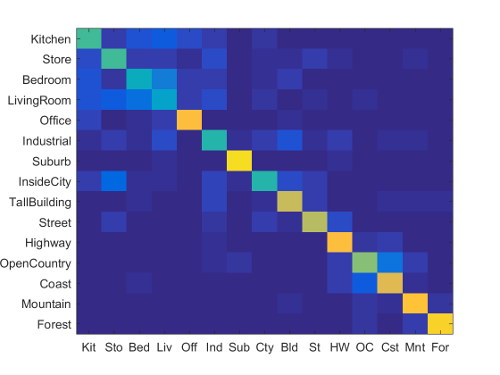
Moving on, the red bars on the far right show the result of combining all of the Bells & Whistles work together in one run. As expected, the combination including RBF yields a worse result than the combination that omits it (left red bar v. right red bar). Also, the far right red bar (inclusion of everything except RBF with the baseline) yields a higher accuracy than any of its components achieve alone. This far right bar is my final implementation/my best result. I show the corresponding confusion matrix to this final implementation/best result below:
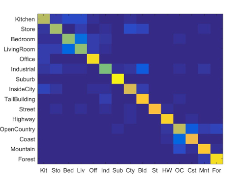 (Accuracy: 78.80%. Vocab Size: 600. SIFT_Size: 6. SIFT_Step: 10. Lambda: 0.0001. Includes Spatial Pyramid,
Kernel Codebook Encoding, and GIST)
(Accuracy: 78.80%. Vocab Size: 600. SIFT_Size: 6. SIFT_Step: 10. Lambda: 0.0001. Includes Spatial Pyramid,
Kernel Codebook Encoding, and GIST)
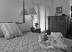
Note also that even with my best implementation, there is still high variance in accuracy across categories. While many of the categories from office onwards have good accuracy, Kitchen, Store, Bedroom and LivingRoom all still have less than desirable accuracy (in fact, even Industrial can also be grouped into this poor accuracy group). I suspect the reason for this is that these categories can look very different. For example, some bedrooms might contain chairs, dressers, bedside tables, bedframes, etc., while other bedrooms may contain some or none of these objects. Contrast that with Forest (one of my highest accuracy categories), where every Forest image almost certainly just contains some combination of trees. Thus, it looks like my best result is understandably unable to deal well with categories whose images can have high variance in how they look/what they include.
As a last point, I think it's worth indicating just how much GIST seems to have helped my result. The inclusion of GIST on the baseline implementation alone yielded 76%, and my final result has an accuracy of 79% (technically 78.80%). Thus, in some ways I start to wonder if the inclusion of additional 'orthogonal' features might be much more valuable than slight implementation changes using one feature. Intuitively at least, this seems to make sense.
Here's the scene classification results visualization for my best implementation:
Accuracy (mean of diagonal of confusion matrix) is 0.788
| Category name | Accuracy | Sample training images | Sample true positives | False positives with true label | False negatives with wrong predicted label | ||||
|---|---|---|---|---|---|---|---|---|---|
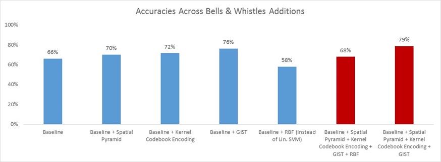
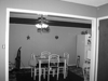
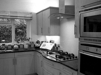
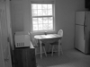
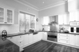
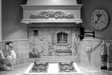
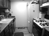
| Kitchen | 0.670 | 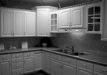 |
 |
 |
 |
 Industrial |
 InsideCity |
 Bedroom |
 Mountain |
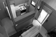
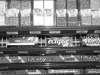
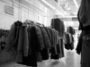
| Store | 0.690 | 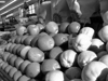 |
 |
 |
 |
 LivingRoom |
 Kitchen |
 TallBuilding |
 InsideCity |
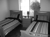
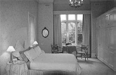
| Bedroom | 0.700 |  |
 |
 |
 |
 Kitchen |
 Kitchen |
 Office |
 Industrial |
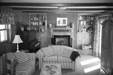
| LivingRoom | 0.600 | 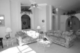 |
 |
 |
 |
 Bedroom |
 Kitchen |
 Bedroom |
 Bedroom |
| Office | 0.930 |  |
 |
 |
 |
 LivingRoom |
 LivingRoom |
 Kitchen |
 Kitchen |
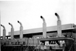
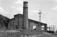
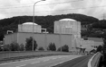
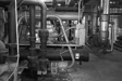
| Industrial | 0.610 |  |
 |
 |
 |
 Bedroom |
 Street |
 Store |
 Store |
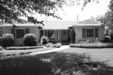
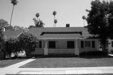
| Suburb | 0.980 | 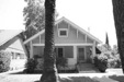 |
 |
 |
 |
 Industrial |
 OpenCountry |
 LivingRoom |
 Store |
| InsideCity | 0.700 |  |
 |
 |
 |
 Industrial |
 Highway |
 Industrial |
 Kitchen |
| TallBuilding | 0.860 |  |
 |
 |
 |
 Industrial |
 Store |
 Coast |
 Industrial |
| Street | 0.850 |  |
 |
 |
 |
 Industrial |
 Kitchen |
 Highway |
 LivingRoom |
| Highway | 0.880 |  |
 |
 |
 |
 Coast |
 OpenCountry |
 OpenCountry |
 Coast |
| OpenCountry | 0.720 |  |
 |
 |
 |
 Coast |
 Mountain |
 Coast |
 Coast |
| Coast | 0.860 |  |
 |
 |
 |
Highway |
 OpenCountry |
 OpenCountry |
 OpenCountry |
| Mountain | 0.840 |  |
 |
 |
 |
 OpenCountry |
 Store |
 OpenCountry |
 OpenCountry |
| Forest | 0.930 |  |
 |
 |
 |
 OpenCountry |
 OpenCountry |
 Store |
 Mountain |
| Category name | Accuracy | Sample training images | Sample true positives | False positives with true label | False negatives with wrong predicted label | ||||