Wengling Chen

Basic Implementation

Tiny Images

The tiny image features are very simple: just use imresize() to shrink each image to 16x16 size, and then normalize the resulting features.

Bag of SIFT

This is slightly more complicated: first we need to build vocabulary. By using vl_dsift(), we get a bunch of sift features out of each image. After that, we use k-means to get the actual "vocabulary".
This vl_dsift() function has several parameters we can change. I choose bin size to be 8 and step size to be 4 or 8 when building the vocabulary, because a small step size will make the sift features more accurate. When calculating bags of sift features for all images, I change step size to 8 because it will make the calculation a little faster.
In the k-means step, k is equal to pre-defined vocabulary size. The choices of vocabulary size will be discussed later in extra credit part.

Linear SVM

Because I used 1-NN in nearest neighbor, there is not much to say about that. Here I will discuss my linear SVM implementation.
This implementation uses 1-vs-all SVMs to classify each sample, and as there are 15 classes, we need to compute 15 SVMs. Each SVM will decide whether a sample belongs to a certain class and give out a number. The sample will finally belongs to the class which its corresponding SVM gives out the largest number.

This linear SVM uses the function vl_svmtrain(). There is something interesting: if we set labels to -1s and 1s, the SVM will actually performs a little better than if we set labels to 0s and 1s. I suppose this is because of the implementation of this specific SVM.
There is another parameter, lambda, which we can play with in this function. I do not tune it too precisely, but rather roughly tested several values by intuition. Finally I go with lambda = 0.00005, which gives me a quite good result. The actual accuracy is discussed in later sections.

Accuracy/Performance Report

The first table shows accuracies based on the whole dataset(i.e. combination of all images in training and test folder). All samples are randomized.
The last result(Bag of SIFT + SVM w/ Gaussian/RBF kernel, vocab_size = 5000) is trained and tuned using k-fold cross-validation and the final accuracy is calculated on a separate validation set.

Method	Accuracy
Tiny Image + Nearest Neighbor Classifier	23.9%
Bag of SIFT + Nearest Neighbor Classifier	55.7%
Bag of SIFT + Linear SVM Classifier	71.9%
Bag of SIFT + SVM w/ Gaussian/RBF kernel, vocab_size = 200	73.7%
Bag of SIFT + SVM w/ Gaussian/RBF kernel, vocab_size = 5000	79.6%

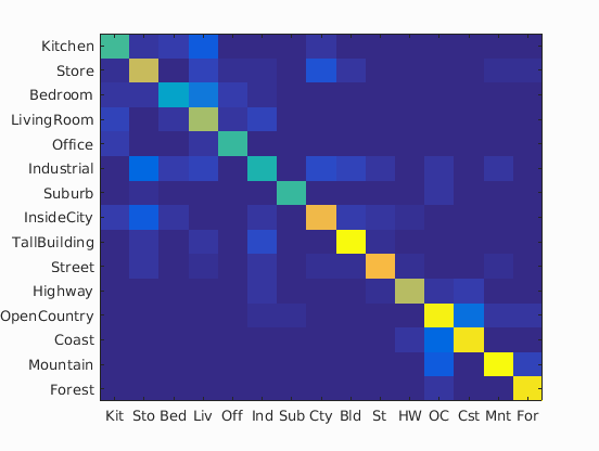
The second table shows the performance and setup of the first three conditions runs on the original 100 sample per class data set, which required by grading rubric:

Method	Confusion Matrix	Accuracy	Execution Time	Parameters
Tiny Image + Nearest Neighbor Classifier		21.7%	19.6s	vocab_size=100; 16x16; Normalized; 1-NN
Bag of SIFT + Nearest Neighbor Classifier		50.3%	36.6s	vocab_size=100; SIFT: size=8, step=8; 1-NN
Bag of SIFT + Linear SVM Classifier		65.7%	59.9s	vocab_size=100; SIFT: size=8, step=8; Linear SVM: Lambda = 0.00005

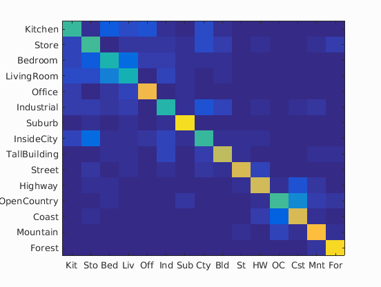
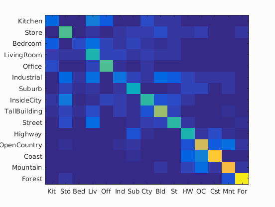
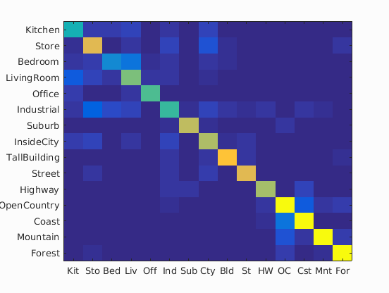
And here is the auto-generated confusion matrix and table for the best result(Bag of SIFT + SVM w/ Gaussian/RBF kernel, vocab_size = 5000):

Accuracy (mean of diagonal of confusion matrix) is 0.796

Category name	Accuracy	Sample training images		Sample true positives		False positives with true label		False negatives with wrong predicted label
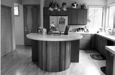
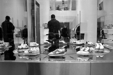
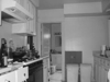
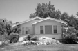
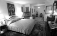
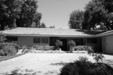
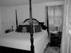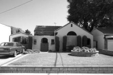
Kitchen	0.345					Industrial	Bedroom	Bedroom	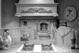Store
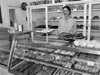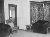
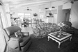
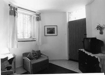
Store	0.892					Bedroom	LivingRoom	LivingRoom	TallBuilding
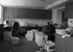
Bedroom	0.345					Office	Kitchen	LivingRoom	LivingRoom
LivingRoom	0.579		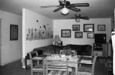			Kitchen	Kitchen	Mountain	Bedroom
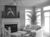
Office	0.446					LivingRoom	LivingRoom	Kitchen	LivingRoom
Industrial	0.579					LivingRoom	Store	Store	Coast
Suburb	0.791					Bedroom	Industrial	Industrial	OpenCountry
InsideCity	0.780					TallBuilding	Store	Bedroom	LivingRoom
TallBuilding	1.114					Street	Highway	LivingRoom	Industrial
Street	0.880					Highway	InsideCity	TallBuilding	InsideCity
Highway	0.758					Coast	Street	OpenCountry	Coast
OpenCountry	1.070					Coast	Highway	Forest	Coast
Coast	1.126					InsideCity	Highway	OpenCountry	OpenCountry
Mountain	1.148					Coast	Industrial	Bedroom	OpenCountry
Forest	1.092					OpenCountry	OpenCountry	OpenCountry	OpenCountry
Category name	Accuracy	Sample training images		Sample true positives		False positives with true label		False negatives with wrong predicted label

Extra Credits

Train the SVM with more sophisticated kernels

Besides the linear SVM, I also used an SVM classifier with Gaussian/RBF kernel. I did this with the widely used LIBSVM. I choose to use C-SVM which makes classifications easier, and also use Gaussian/RBF kernel.
There are two parameters, gamma and penalty parameter C, which we can tune. In the cross-validation section I will discuss how I choose them.
As shown before, using a Gaussian/RBF kernel can improve the accuracy from about 70% to 79%, which is quite good.

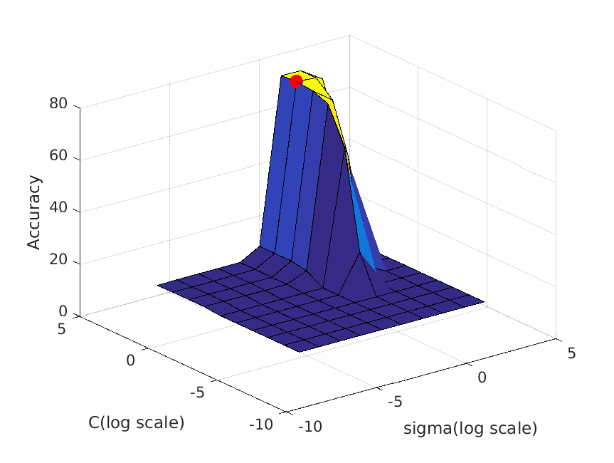
Use cross-validation to measure performance

I used k-fold cross-validation to tune my parameter sigma(which is related to gamma: gamma = 1/(2*sigma^2)) and penalty parameter C in my RBF SVM. Instead of the proposed way on assignment webpage, I used the "traditional" way, in which I just divided the whole training set randomly into k parts with roughly equal sizes. This makes it much longer to compute, though.
The values of sigma and C I tried are the following: [0.001, 0.003, 0.01, 0.03, 0.1, 0.3, 1, 3, 10, 30]. As you may realize, this is roughly a geometric sequence with a factor of 3, and practice shows this is quite effective. Because there are two variables, altogether I will try 10^2 = 100 combinations, and because I choose k=12 in k-fold cross-validation, I will compute 100*12 = 1200 models every time. This is definitely a lot to compute, and because I can only run this on CPU, it takes me some time even if I have parallelized it partially.

Not too surprising, the result is quite uniform when I tried to get the best parameter under different vocabulary sizes: almost every time the best sigma is 1, and the best C is often 3, 10 or 30.
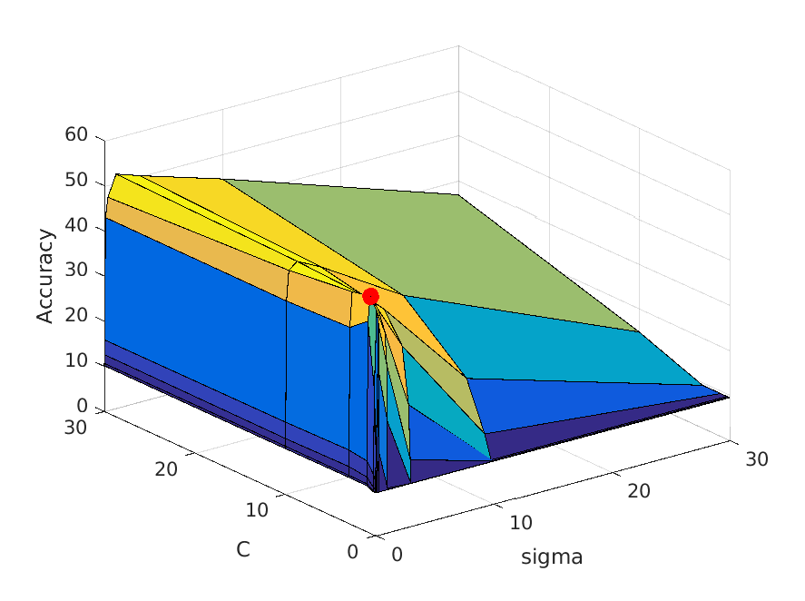
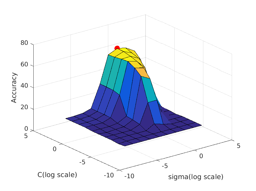
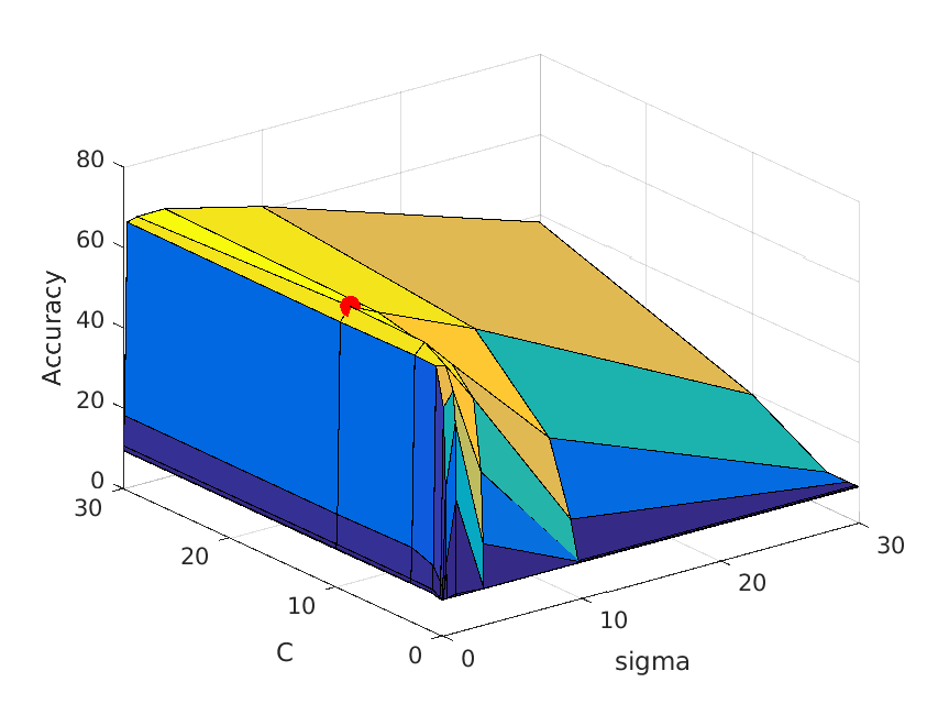
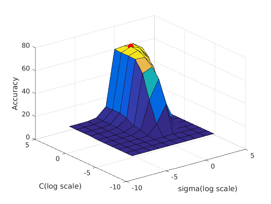
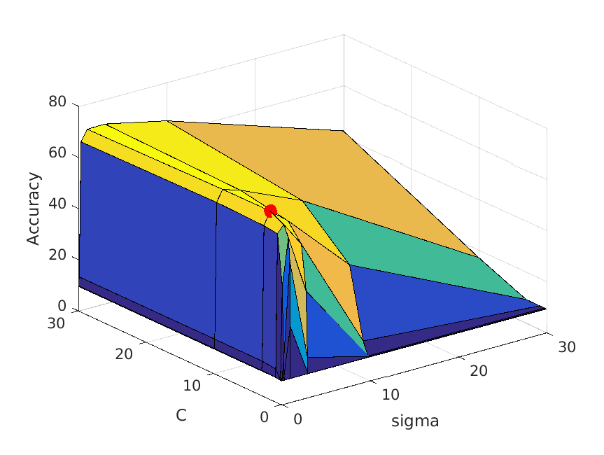
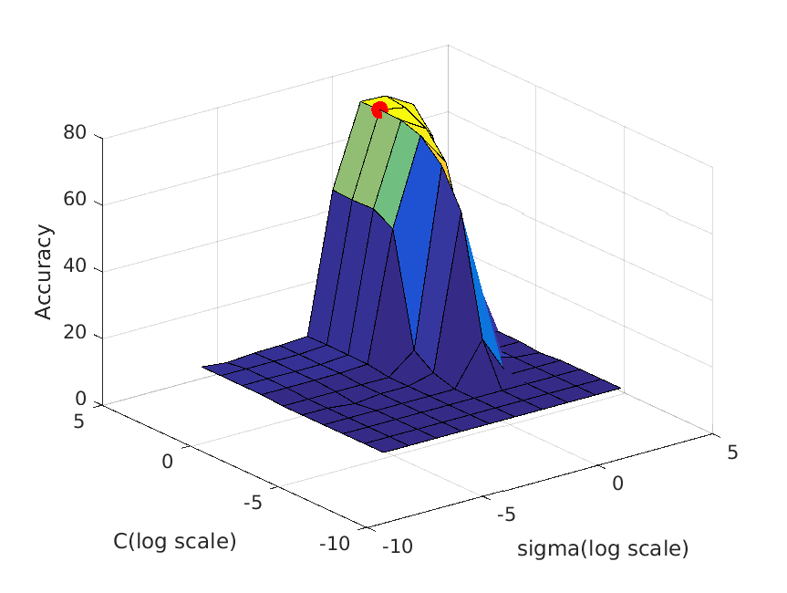
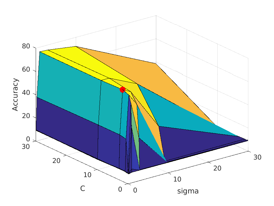
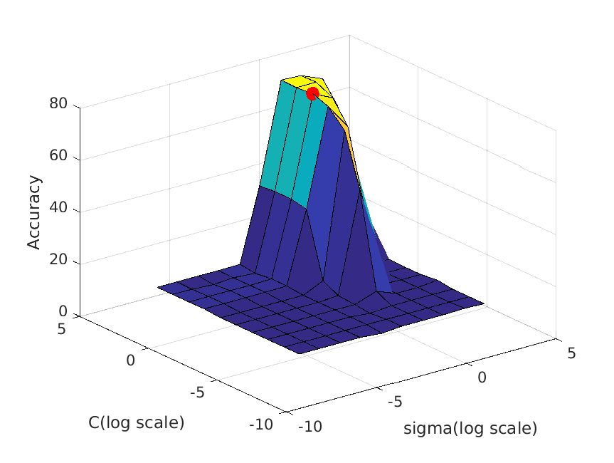
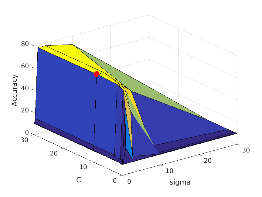
The following table shows a visualization of average accuracies by cross-validation when tuning parameters. I forgot to save the accuracies, so I cannot show the exact accuracies at the time these graphs are calculated, but you can definitely get some ideas from the graph:

vocab_size=10. Best at sigma=0.3, C=1, accuracy is roughly 54%

vocab_size=20. Best at sigma=1, C=30, accuracy is roughly 62%

vocab_size=50. Best at sigma=1, C=10, accuracy is roughly 67%

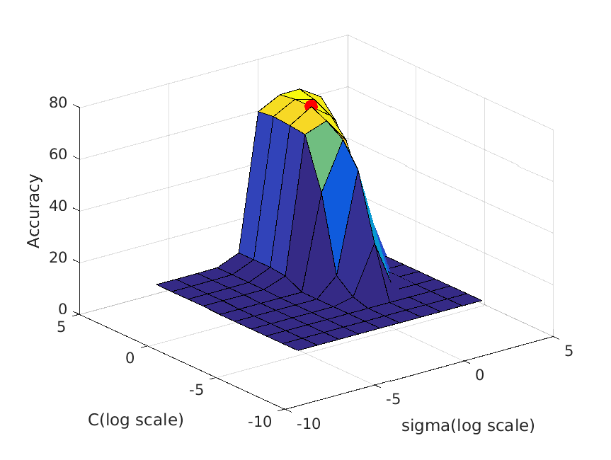
vocab_size=100. Best at sigma=1, C=3, accuracy is roughly 71%

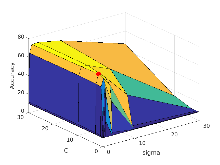
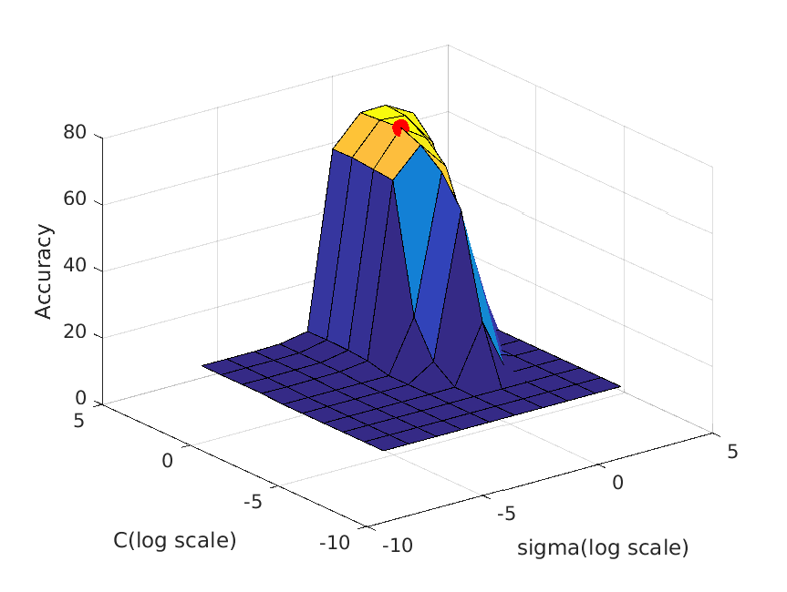
vocab_size=200. Best at sigma=1, C=3, accuracy is roughly 73%

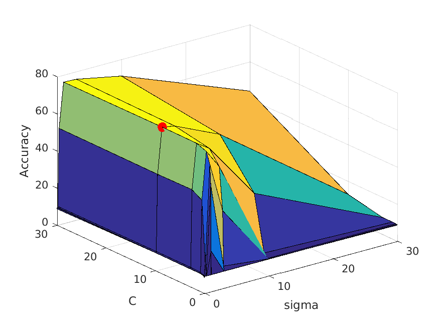
vocab_size=400. Best at sigma=1, C=10, accuracy is roughly 77%

vocab_size=1000. Best at sigma=1, C=3, accuracy is roughly 77%

vocab_size=5000. Best at sigma=1, C=10, accuracy is roughly 79%

Add a validation set to your training process to tune learning parameters

I cut out 30% of the whole dataset as a validation set to evaluate the performance of the chosen vocabulary size. (Actually this method is also used when tuning sigma and C, but in that process I only use the validation set to see the final performance rather than actually "tuning" sigma and C) Nonetheless, this validation set is just a randomly chosen 30 percent samples of the whole set, and it is used to make sure the model is not overfitting. By using the validation set, I still get a high accuracy with my models, which shows that they are well generalized. The actual accuracy I got on validation set with different vocabulary sizes will be shown in the next section.

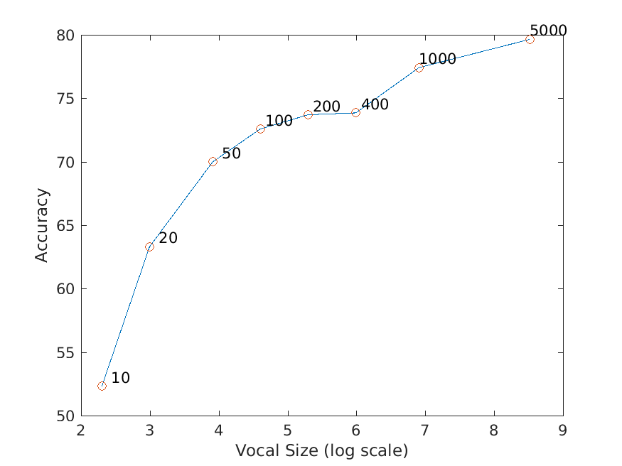
Experiment with many different vocabulary sizes and report performance

I experimented on the following vocabulary sizes: 10, 20, 50, 100, 200, 400, 1000 and 5000. 10000 is too big for my machine to calculate.
The result is as I expected: the larger the vocabulary size is, the higher the accuracy will be.

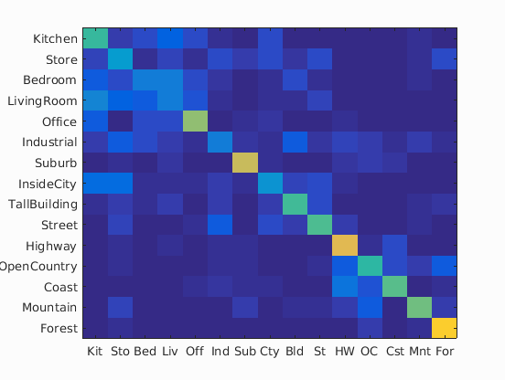
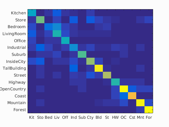
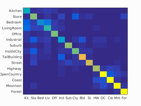
In the following table is the confusion matrices with different values of vocabulary sizes, and also its accuracy on a separate validation set:

Vocabulary Size	Confusion Matrix	Accuracy
10		52.3%
20		63.3%
50		70.0%
100		72.6%
200		73.7%
400		73.8%
1000		77.4%
5000		79.6%

And here is a visualization of the relationship between vocabulary size and accuracy. For clarity, vocabulary sizes are plotted on logarithmic scale: