Project 4 / Scene Recognition with Bag of Words
Example of scene recognition using bag of words (nearest neighbor).
To start out with this assignment I first implemented tiny image representation. In tackling this problem I first found the number of rows in the image path. I then proceeded to iterate through the rows reading each image path to get the image. I then resized it to a 16 by 16. To improve performance I then normalized image the image body. I did this by first finding the mean the transpose made into a 1x256 matrix and subtracted and divided it by itself in order to normalize my data. After coding the tiny image I could not test it until I finished nearest neighbor as the placeholder classifier only gave me 6% accuracy. I did notice that the tiny image representation calculations happened almost instaneously which I attribute to the image having a low amount of features as well as just the image reading process itself is a lot less intensive for functions to run.
Below I have a code snipet showing how I did the normalization for the image. This is done by subtracting the mean and dividing by the norm.
	%normalizing
       meanVector = mean(reshape(temp',[1,256]));
       vector = (reshape(temp',[1,256]) - meanVector) / norm((reshape(temp',[1,256]) - mean));
       image_feats(count, :) = vector;
The next step of my coding process, I proceeded to implement nearest neighbor. This process was relatively straight forward as Ie were given the matrices holding the train_image_feats. I first tried implementing nearest neighbor using pdist2 function, but I realized that Matlab's vl_alldist2 was great at calculating the distances between possible features. After the set of distances have been calculated the nearest neighbor was easily found by sorting the matrix and returning the first index. Looking back at my code this could probably be improved by just calculating the min, so the sorting step does not even have to happen. Ultimately I chose the sort method because if I wanted multiple nearest neighbors to help in calculation, the sort method quickly became a much better choice in returning the answer. Once I was able to finish nearest neighbor I was able to test my tiny image to see if it correctly worked the way I had expected. Combining the two I was able to get above 20% accuracy which I was quite proud of. The huge improvement using nearest neighbor mainly stems from the power it holds. The algorithm does not require and training and therefore runs in a lot less time not neededing to go through a training set before going to an exactual testing set. The nearest neighbor however is not without its faults as images with more noise seem to be a hindrance to the nearest neighbor algorithm. The algorithm itself does not take in dimensionality that well and can not tell which dimensions do not help in the calculation. The image below shows confusion matrix as well as a link which shows the categories each thumbnail image fell in. Looking at the false positives and false negatives the tiny/nn seems to do well with very dinstinct images such as highways and street, but suffers from more cluttered enviorments such as the kitchen. Perhaps the nn does not take into account the dimensionaty and some dimensions are no suitable for helping categorize the images.
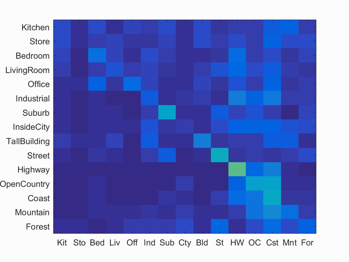
Example of scene recognition using tiny image representation (nearest neighbor).
For the next part I implemented the build vocabulary function. As I are progressing into the bag of sift features I need a vocabulary in order to see all the visual words. In terms of the step size to sample I first tested it with a step size 5, but when I tried it later on with the sift function the processing time was too long, so I increased it to 10. In implementing the vocabulary I first made got the numer of rows of the image paths and using that I iterated over the rows reading the image and then performing a sift. A really helpful function I found for this part of the process was the vl_dsift function. It took alot of playing around with different step size and parameters until I was able to get one I was happy with. For debugging purposes I used the fast parameter that is built into vlsift that helped a lot with debugging my code. After I had stored the large amount of features, I then group it using kmean clustering. A very helpful function I found to help with this was the vl_kmeans function. I determined the number of clusters by the vocab size. The reason I save the vocab data itself is becuase if I save the cluster of centroids I can use it later to avoid recomputing it.
Here is a example of a snippet of code I used to help create sift_features with the help of vl_dsift
[~, sift_feats] = vl_dsift(single(imread(image_paths{count})), 'step', 10);
After implementing the build_vocabulary function, I then proceeded to implement the get_bags_of_sifts function. By first getting the row size of the image paths I can again iterate through the rows. Similar to the function in vocab, I first got the sift features using the helpful vld_sift function. I played around with different step sizes before choosing a step size of 20. I found that usually anything lower would greatly increase the processing the time. From the features I then found the distances between them and used the sorted matrix to create a histogram. The histogram takes in distinct parameters. After a lot of playing around to see what numbers worked, I found that nmy combination seemed to give the best result in terms of both accuracy and performance. The histogram is then divided by the norm of the histogram and is stored in image feature. The advatages of this approuch over the tiny image is many. The large amount of SIFT descripters allow me to be able to cluster them based off the vocabulary I made earlier. By allowing the histogram to represent as manyu dimensions as the number of vocab words, the normalized histogram is able to represent a lot more information then the tiny image function. As for the results after I ran the nearest neighbor classification on my bag of SIFTs I was able to get quite a large increase in accuracy. The accuracy was able to go over 50% which I largely attribute to the vocabulary enable the many SIFT descripters to be grouped into better image features. This allowed nearest neighbor to have a higher degree of accuracy as the features themselves represented the image better. The large number of feature points also helped in strenghthing the accuracy of the result, but at the cost of a much larger run time approximation. Using the vocab as well as SIFT has greatly improved the performance of the Forest and Suburb, perhaps the spitting and help of the SIFT descripters help identify key differences to seperate them. Notably most of the accuracy have increased but the bedroom and living room still have a hard time correctly identifying.
Here is a code snippet that shows how I read the image after obtaining the rows and then sort it by distance for histograms later. The confusion matrix and a link to the true/false positive/negative is found behind it.
	[~, sift_feats] = vl_dsift(single(imread(image_paths{count})), 'step', 20);

	distances = vl_alldist2(single(sift_feats), vocab);
	%sort the distances
	[~, i] = sort(distances, 2);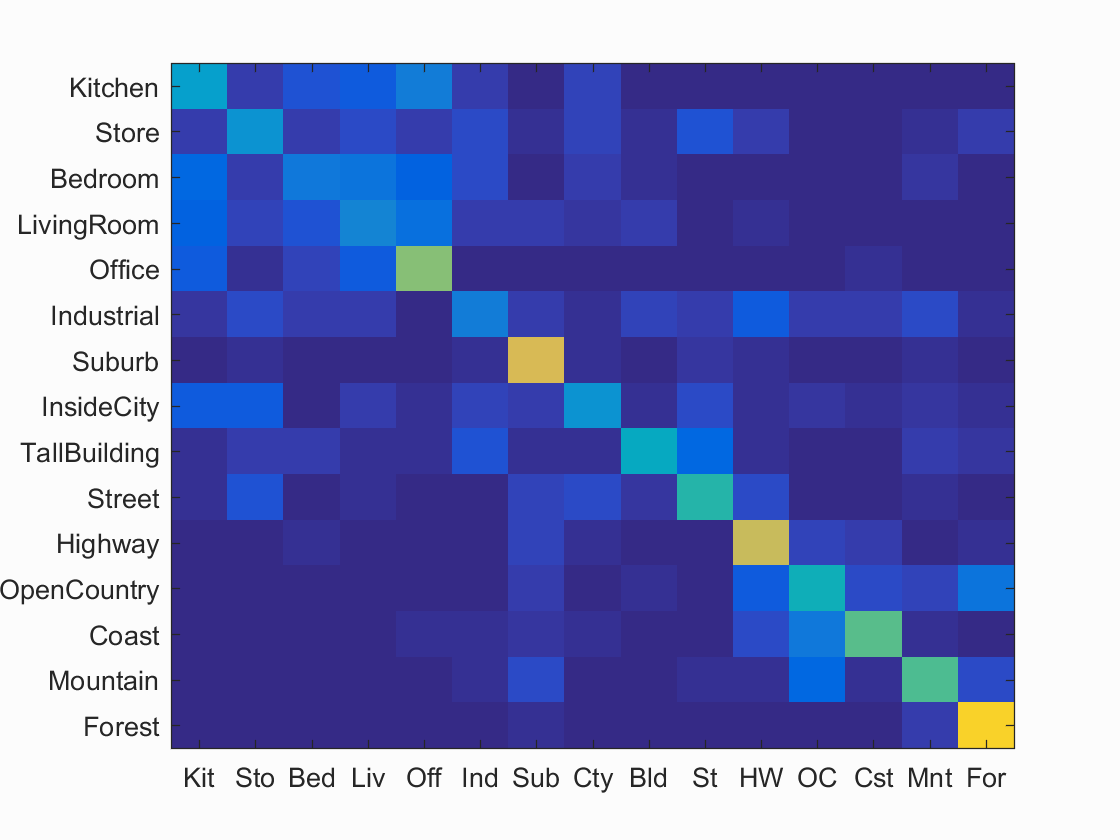
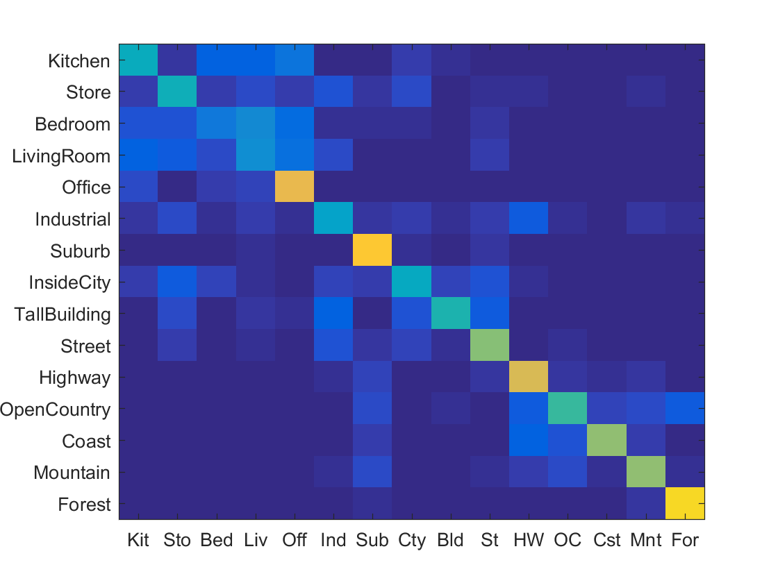
Example of scene recognition using bag of sifts (nearest neighbor).
Finally for the final part of the project, I implemented the svm_classify function. I first got the category list as well as the length of the list. Using this information. I iterated through the categories checking if the category given and the label matched which was used to create binary groupings. By grouping the values together I was then able to use the very helpful vl_svmtrain that helped me calculate the w and b values. After all categories have been finished I then calculated the confidence level using the image features with w and b values. The SVM algorithm itself performs better then its counterpart the nearest neighbor because it the feature space itself is divided into hyperplanes allowing for a better categorizatoin of data. The biggest difference between the two is that the SVM is able to learn which dimensions are useful in calculating groupings. This allows my calcultions to be alot more accurate. If you want more information about the accuracy feel free to look at the links throughout the report that shows the groupings based off thingys such as false positivies etc. In terms of the results the bedroom had a notable improvement over nearest neighbor. The living however was still having similar problems identifying the images. The SVM definitly helped identify key features that helped seperate the bedroom from the office or living room.
Here is a code snippet showing how I calculated the confidance.
	confi = bb(ones(m, 1),:) + ww * test_image_feats ;
	[~, i] = max(confi');
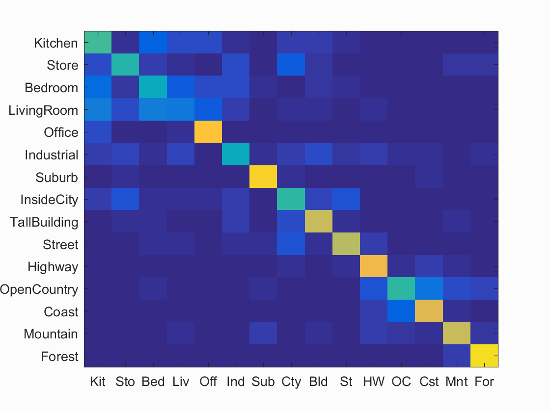
Example of scene recognition using bag of sifts (SVM).