Weiyang Liu

Basic Experiments

1. Tiny images plus nearest neighbor classifier

I implemented the tiny images features and then normalized them. The code is as follows:

% get tiny images features from raw images
function image_feats = get_tiny_images(image_paths)
    num = size(image_paths,1);
    rows = 16;
    cols = 16;
    for i = 1:num
        img = imread(image_paths{i});
        resize_img = imresize(img, [rows cols]);
        image_feats_m(i,:) = reshape(resize_img,[1 rows*cols]);
        image_feats(i,:) = double(image_feats_m(i,:));
        image_feats(i,:) = image_feats(i,:) - repmat(mean(image_feats(i,:)),...
            size(image_feats(i,:),1),size(image_feats(i,:),2));
        image_feats(i,:) = image_feats(i,:)/norm(image_feats(i,:),2);
    end
 end

Then I implemented the nearest neighbor classifier (1-NN). The code is as follows:

% 1-NN classifier
function predicted_categories = nearest_neighbor_classify(train_image_feats, train_labels, test_image_feats)
    D = vl_alldist2(train_image_feats',test_image_feats','L2');
    [~,idx] = sort(D,'ascend');
    % 1-nn
    idx_min = idx(1,:);
    predicted_categories = cell(size(test_image_feats,1),1);
    for i = 1:size(test_image_feats,1)
        predicted_categories{i} = train_labels{idx_min(i)};
    end
end

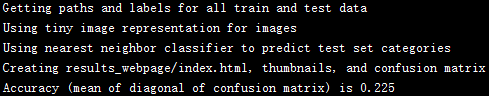
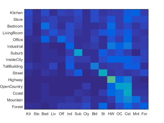
Combining the tiny images and 1-NN classifier, I achieved 22.5% accuracy. The confusion matrix is shown as follows:

2. Tiny images plus linear SVM classifier

I implemented the linear SVM classifier. The code is as follows:

% linear SVM classifier
function predicted_categories = svm_classify(train_image_feats, train_labels, test_image_feats)
    categories = unique(train_labels); 
    num_categories = length(categories);
    LAMBDA = .0001;
    for i = 1:num_categories
        matching_indices = strcmp(categories{i}, train_labels);
        matching_indices = double(matching_indices);
        matching_indices(find(matching_indices==0)) = -1;
        svm_train_labels = double(matching_indices);
        [w(:,i),b(i,1)] = vl_svmtrain(double(train_image_feats'), svm_train_labels, LAMBDA);
    end
    confidence = exp(w'*test_image_feats'+ repmat(b,1,size(test_image_feats,1)));
    [~,idx] = max(confidence);
    for i = 1:size(test_image_feats,1)
        predicted_categories{i,1} = categories{idx(i)};
    end
 end

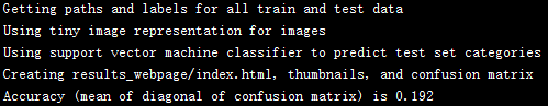
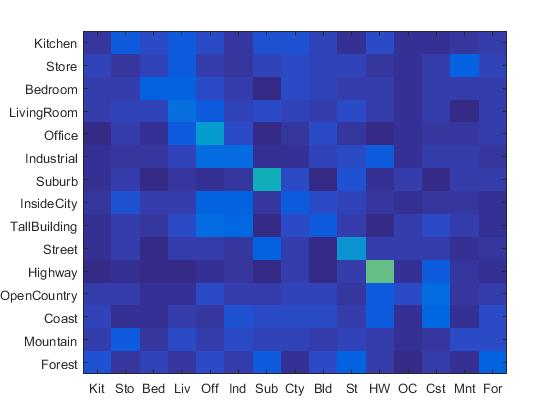
Combining the tiny images and linear SVM classifier, I achieved 19.2% accuracy. The confusion matrix is shown as follows:

3. SIFT BoW features plus 1-NN classifier

I implemented the SIFT BoW features via two steps. First, I set the size of the vocabulary as 200, and constructed the vocabulary using the following code:

% bulid vocabulary for SIFT descriptors
function vocab = build_vocabulary( image_paths, vocab_size )
    SIFT_features = [];
    for i = 1:size(image_paths,1)
        img = single(imread(image_paths{i}));
        [~, SIFT_features_delta] = vl_dsift(img,'fast','Step',8,'Size',8);
        SIFT_features = [SIFT_features,SIFT_features_delta];
    end
    [centers, ~] = vl_kmeans(single(SIFT_features), vocab_size);
    vocab = centers';
 end

Second, I constructed the histogram features using the vocabulary and the SIFT descriptors from training and testing images. The code is as follows:

% get bags of sifts features
function image_feats = get_bags_of_sifts(image_paths)
    load('vocab.mat')
    image_feats = [];
    vocab_size = size(vocab, 1);
    for i = 1:size(image_paths,1)
        img = single(imread(image_paths{i}));
        [~, SIFT_features] = vl_dsift(img,'Fast','Step',8,'Size',8) ;
        D = vl_alldist2(vocab',single(SIFT_features)); 
        [~,idx] = sort(D);
        idx_min = idx(1,:);
        unit_vec = eye(vocab_size);
        sift_hist = sum(unit_vec(idx_min,:),1);
        image_feats(i,:) = sift_hist./norm(sift_hist,2);
    end
end

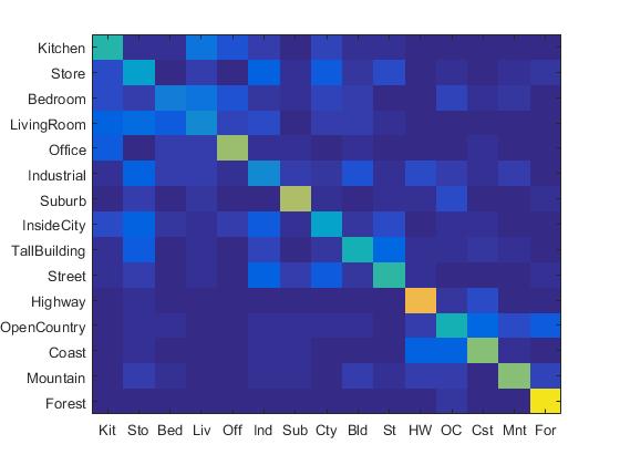
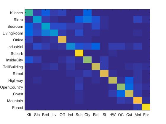
Combining the SIFT BoW features and 1-NN classifier, I achieved 50.8% accuracy. The confusion matrix is shown as follows:

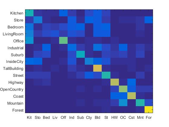
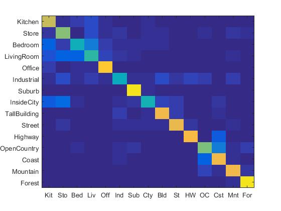
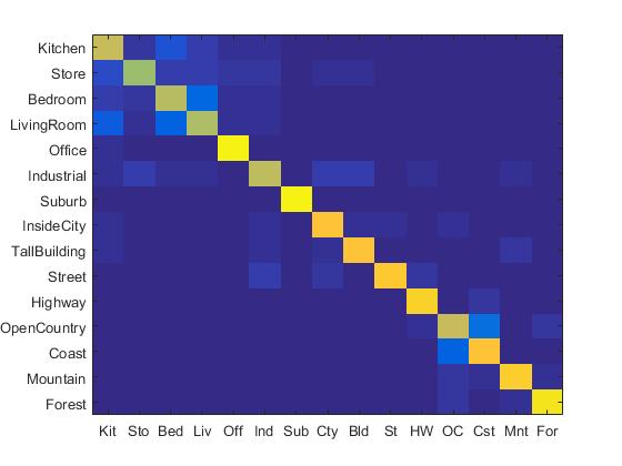
4. SIFT BoW features plus linear SVM classifier

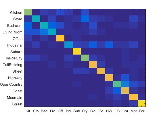
Combining the SIFT BoW features and linear SVM classifier, I achieved 67.3% accuracy. The confusion matrix is shown as follows:

Some samples from the recognition are shown as follows:

Category name	Accuracy	Sample training images		Sample true positives		False positives with true label		False negatives with wrong predicted label
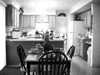
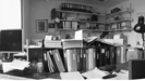
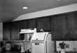
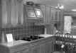
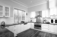
Kitchen	0.620					Bedroom	LivingRoom	TallBuilding	Bedroom
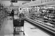
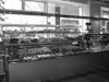
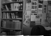
Store	0.520		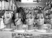			LivingRoom	Bedroom	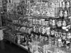Forest	Office
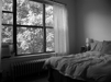
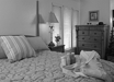
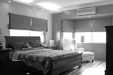
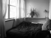
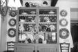
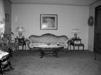
Bedroom	0.410		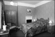		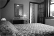	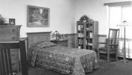LivingRoom	LivingRoom	Kitchen	LivingRoom
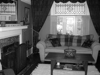
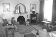
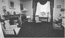
LivingRoom	0.430					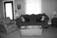Industrial	Bedroom	Bedroom	Kitchen
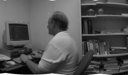
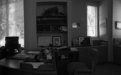
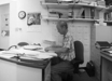
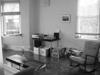
Office	0.810					InsideCity	Bedroom	Bedroom	LivingRoom
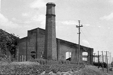
Industrial	0.420		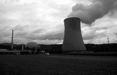			Suburb	TallBuilding	Kitchen	TallBuilding
Suburb	0.890		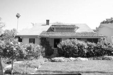			InsideCity	OpenCountry	OpenCountry	LivingRoom
InsideCity	0.410					TallBuilding	Industrial	Store	Kitchen
TallBuilding	0.710					Office	InsideCity	Industrial	Industrial
Street	0.790					OpenCountry	Bedroom	InsideCity	Store
Highway	0.830					Mountain	Street	Coast	Office
OpenCountry	0.550					Coast	Industrial	Mountain	Mountain
Coast	0.780					OpenCountry	Mountain	Highway	Highway
Mountain	0.820					Store	Store	Coast	Forest
Forest	0.950					TallBuilding	OpenCountry	Mountain	Mountain
Category name	Accuracy	Sample training images		Sample true positives		False positives with true label		False negatives with wrong predicted label

Extra Credits

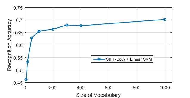
1. Experiment with many different vocabulary sizes (3pts)

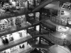
I experimented with many different vocabulary sizes such as 10, 20, 50, 100, 200, 300, 400, 1000. Their confusion matrix are shown as follows. (The first row: 10, 20, 50, 100 (from left to right). The second row: 200, 300, 400, 1000 (from left to right).)

I also plot an "accuracy vs. vocabulary size" figure, as shown in the following:

2. Using RBF kernel for nonlinear SVM (3pts)

I implemented the non-linear SVM with RBF kernel using the MATLAB built-in svmtrain function. The code is as follows:

% non-linear SVM with RBF kernel
function predicted_categories = nonlinear_svm_classify(train_image_feats, train_labels, test_image_feats)
    categories = unique(train_labels); 
    num_categories = length(categories);
    LAMBDA = .0004;
    for i = 1:num_categories
        matching_indices = strcmp(categories{i}, train_labels);
        matching_indices = double(matching_indices);
        matching_indices(find(matching_indices==0)) = -1;
        svm_train_labels = double(matching_indices);
        svm_model{i} = fitcsvm(double(train_image_feats), svm_train_labels, 'KernelFunction','rbf');
    end
    for i = 1:num_categories
        [~,scores] = predict(svm_model{i},test_image_feats);
        confidence(i,:) = (scores(:,2))';
    end
    [~,idx] = max(confidence);
    for i = 1:size(test_image_feats,1)
        predicted_categories{i,1} = categories{idx(i)};
    end
end

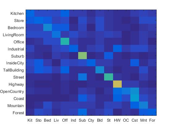
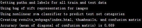
I tested the nonlinear SVM with tiny images and SIFT-BoW features. The results for tiny images are shown as follows:

The results for SIFT-BoW features are shown as follows:

We can see both results are higher than the linear SVM.

3. GIST descriptor (5pts)

I implemented the GIST features with the extra LMgist.m and imresizecrop.m downloaded from the GIST project page. My code is as follows:

% GIST descriptor
function image_feats = get_gist_vector(image_paths)
    image_feats = [];
    clear param
    for i = 1:size(image_paths,1)
        img = single(imread(image_paths{i}));
        param.imageSize = [256 256];
        param.orientationsPerScale = [8 8 8 8]; % number of orientations per scale
        param.numberBlocks = 4;
        param.fc_prefilt = 4;
        image_feats(i,:) = LMgist(img, '', param);
    end
end

For the proj4.m file, I added the following part to the feature extraction section:

% *******************extra credit (GIST)******************
    case 'gist descriptor'
        train_image_feats = get_gist_vector(train_image_paths);
        test_image_feats = get_gist_vector(test_image_paths);
        save('gist_features.mat', 'train_image_feats','test_image_feats');
        % load('gist_features.mat');
% ****************end of extra credit (GIST)***************

If I only used GIST and linear SVM, I can obtain the following results:

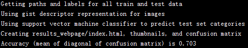
If I simply concatenated GIST to the SIFT-BoW features and used linear SVM,, I can obtain the following results:

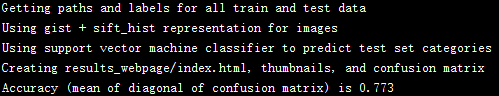
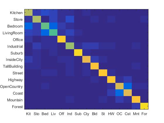
4. Fisher Encoding (5pts)

I implemented the fisher encoding via two steps. First, I constructed a vocabulary with Gaussian mixture model. The code is as follows:

% build GMM vocabulary
function [means, covariances, priors] = build_GMM_vocabulary( image_paths, numClusters )
    SIFT_features = [];
    for i = 1:size(image_paths,1)
        img = single(imread(image_paths{i}));
        [~, SIFT_features_delta] = vl_dsift(img,'fast','Step',8,'Size',8);
        SIFT_features = [SIFT_features,SIFT_features_delta];
    end
    [means, covariances, priors] = vl_gmm(double(SIFT_features), numClusters);
end

Second, I constructed fisher vector using the vocabulary. The code is as follows:

% get fisher vector with the GMM vocabulary
function image_feats = get_fisher_vector(image_paths, means, covariances, priors)
    load('vocab_GMM.mat')
    image_feats = [];
    for i = 1:size(image_paths,1)
        img = single(imread(image_paths{i}));
        [~, SIFT_features] = vl_dsift(img,'Fast','Step',8,'Size',8) ;
        image_feats(i,:) = vl_fisher(double(SIFT_features), means, covariances, priors, 'Improved', 'Fast');
    end
end

Finally, I added some code to the proj4.m file:

% *******************extra credit (Fisher Vector)******************
    case 'sift fisher vector'
        if ~exist('vocab_GMM.mat', 'file')
            fprintf('No existing visual word vocabulary found. Computing one from training images\n')
            numClusters = 256;
            [means, covariances, priors] = build_GMM_vocabulary(train_image_paths, numClusters);
            save('vocab_GMM.mat', 'means', 'covariances', 'priors')
        end
        
        train_image_feats = get_fisher_vector(train_image_paths, means, covariances, priors);
        test_image_feats = get_fisher_vector(test_image_paths, means, covariances, priors);
        save('sift_FV_features.mat', 'train_image_feats','test_image_feats');
        % load('sift_FV_features.mat');
        
        % dimension reduction by PCA
        reduced_dim = 512;
        num_train = size(train_image_feats,1);
        num_test = size(test_image_feats,1);
        [~,new_feats] = pca([train_image_feats;test_image_feats]);
        new_feats = new_feats(:,1:reduced_dim);
        train_image_feats = new_feats(1:num_train,:);
        test_image_feats = new_feats(num_train+1:num_train+num_test,:);
        save('sift_FV_features_PCA.mat', 'train_image_feats','test_image_feats');
        % load('sift_FV_features_PCA.mat');
% ****************end of extra credit (Fisher Vector)***************

Since the dimension of Fisher vector is too large, I also implemented a PCA dimension reduction for Fisher vector. If I directly run linear SVM on top of the original Fisher vector, I obtained the following results:

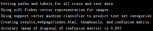
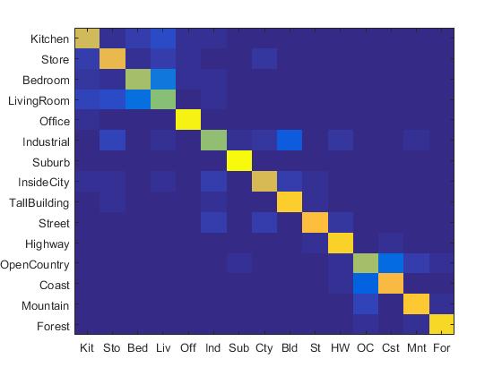
If I used PCA to reduce the dimension of Fisher vector to 512, then I obtained the following results:

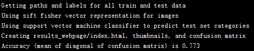
Best Obtained Accuracy

I first reduced dimension of Fisher vector to 512 via PCA and then concatenated GIST to the SIFT fisher vector, constructing fusion features with dimension of 1024. I add the code to the proj4.m file, shown as follows:

% *******************extra credit (GIST+SIFT_fv)******************
    case 'gist + sift_fv'
        if ~exist('vocab_GMM.mat', 'file')
            fprintf('No existing visual word vocabulary found. Computing one from training images\n')
            numClusters = 256; %Larger values will work better (to a point) but be slower to compute
            [means, covariances, priors] = build_GMM_vocabulary(train_image_paths, numClusters);
            save('vocab_GMM.mat', 'means', 'covariances', 'priors')
        end
        train_image_feats = get_fisher_vector(train_image_paths, means, covariances, priors);
        test_image_feats = get_fisher_vector(test_image_paths, means, covariances, priors);
        % dimension reduction by PCA
        reduced_dim = 512;
        num_train = size(train_image_feats,1);
        num_test = size(test_image_feats,1);
        [~,new_feats] = pca([train_image_feats;test_image_feats]);
        new_feats = new_feats(:,1:reduced_dim);
        train_image_feats = new_feats(1:num_train,:);
        test_image_feats = new_feats(num_train+1:num_train+num_test,:);
        train_image_feats_part1 = train_image_feats;
        test_image_feats_part1 = test_image_feats;
        % load('sift_FV_features_PCA.mat');
        % train_image_feats_part1 = train_image_feats;
        % test_image_feats_part1 = test_image_feats;

        train_image_feats_part2 = get_gist_vector(train_image_paths);
        test_image_feats_part2 = get_gist_vector(test_image_paths);
        save('gist_features.mat', 'train_image_feats','test_image_feats');
        % load('gist_features.mat');
        % train_image_feats_part2 = train_image_feats;
        % test_image_feats_part2 = test_image_feats;
        train_image_feats = [train_image_feats_part1,train_image_feats_part2];
        test_image_feats = [test_image_feats_part1,test_image_feats_part2];

        save('gist_sift_hist_features.mat', 'train_image_feats','test_image_feats');
%         load('gist_sift_hist_features.mat');
% ****************end of extra credit (GIST+SIFT_fv)***************

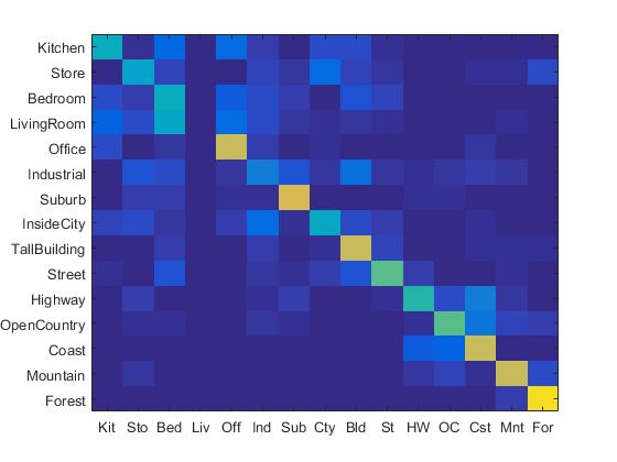
I simply used linear SVM to classify these features and obtained the following results:

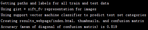
Category name	Accuracy	Sample training images		Sample true positives		False positives with true label		False negatives with wrong predicted label
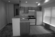
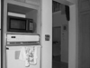
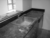
Kitchen	0.730		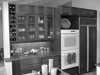			TallBuilding	InsideCity	Store	Bedroom
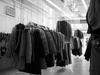
Store	0.650		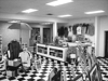			Bedroom	TallBuilding	Highway	TallBuilding
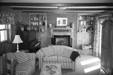
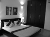
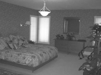
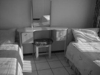
Bedroom	0.690		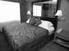			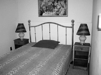LivingRoom	Store	LivingRoom	Kitchen
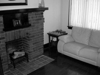
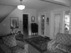
LivingRoom	0.680		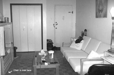			Industrial	Bedroom	Kitchen	Store
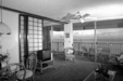
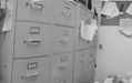
Office	0.980		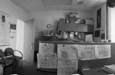			Bedroom	LivingRoom	Kitchen	Kitchen
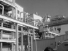
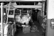
Industrial	0.710		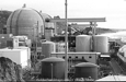		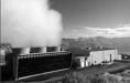	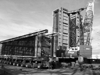InsideCity	InsideCity	TallBuilding	LivingRoom
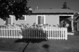
Suburb	0.980		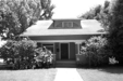		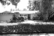			LivingRoom	Kitchen
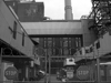
InsideCity	0.850					Highway	Industrial	TallBuilding	Industrial
TallBuilding	0.850					Industrial	InsideCity	Kitchen	Industrial
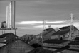
Street	0.860					InsideCity	InsideCity	InsideCity	Industrial
Highway	0.900					Store	Street	Kitchen	LivingRoom
OpenCountry	0.720					Coast	Coast	Coast	Coast
Coast	0.850					OpenCountry	OpenCountry	OpenCountry	OpenCountry
Mountain	0.890					TallBuilding	Forest	Forest	OpenCountry
Forest	0.940					Mountain	OpenCountry	OpenCountry	Mountain
Category name	Accuracy	Sample training images		Sample true positives		False positives with true label		False negatives with wrong predicted label