Project 4 : Scene Recognition with Bag of Words

1. Tiny Images + K Nearest Neighbor
2. Bigs of SIFT + K Nearest Neighbor
3. Bigs of SIFT + 1 vs All Linear SVM
4. Extra credit/Graduate credit

1. Tiny Images + K Nearest Neighbor

Tiny image feature is the simplest feature used in this project. Each image is resize to a 16x16 matrix. Then the matrix is converted to zero mean. The tiny image is not made to have unit length, but each pixel is divided by (3 times standard deviation). At last, each tiny image is reshaped to a row vector. Thus the tiny image feature of all training/testing data is a matrix.

K Nearest Neighbor (KNN) is implemented to classify testing images, given training images with labels. For each testing image, the distances between the testing image feature and all training image features are calculated. The closest K training images are recorded. Among the K training images, there is a most frequent category. Or if some categories show up for the same times, the closest category (based on the feature distance) is taken as the most frequent category. Then the testing image is labeled as the most frequent category.

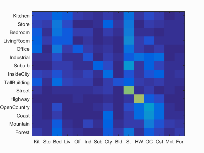
Using tiny image features with KNN classifier, we can classify all the testing images as a base line result. Choosing K = 8, 20.0% accuracy has been achieved. Fig. 1.1 shows the confusion matrix of this method. And Fig. 1.2 indicates how the classifying performance varies with K values. I find that the performace would saturate or even drop at high K.

2. Bags of SIFT + K Nearest Neighbor

In this part, bags of quantized SIFT features are used to represent features of images. A vocabulary of visual words is built by taking randomly sampled SIFT features from training images and clustering them into certain number of clusters. Each cluster represents a visual word. In this process, there are couple parameters designed to sample and extract SIFT features. First, only a number of training images is chosen to extract a number of SIFT features. 150 training images are randomly chosen and then for each image 500 SIFT features are randomly sampled for K-means clustering. The step size in vl_dsift is chosen to be 12. In general, I find that smaller step size for sampling SIFT features could increase classifying accuracy modestly but increase the computational time dramatically. However, the number of vocab_size, i.e. the number of clusters and parameters in extracting SIFT features to build vocabulary features are also important, having large impact on accuracy. As my computer does not have big computational power, the parameters in building vocabulary are chosen for fast computation.

After building vocabulary, training and testing images are represented by histograms of visual words. For each image, feature2samples SIFT features are sampled, and each SIFT feature is classified to nearest K-means cluster center based on the L2 distance. Then for all the SIFT features in one image, they can be counted to each cluster center and form a histogram. The number of bins in the histogram is exactly the vocab_size. Finally each histogram is normalized in case that the number of sampled SIFT features are different from image to image(when the total number of extracted SIFT features is less than feature2samples). There are three parameters in this step, that is, the step size and step in vl_dsift and feature2samples. The step size should be smaller than that in building vocabulary. However, if it is too small, the computational time increases. The step parameter adjusts the sampling density. For feature2samples, it helps increase the classifying accuracy when it is large. However, the accuracy would saturate after feature2samples increases to certain number. And with too many samples in K-means, the speed would be very slow. Here 500 is found to be a good number of features. 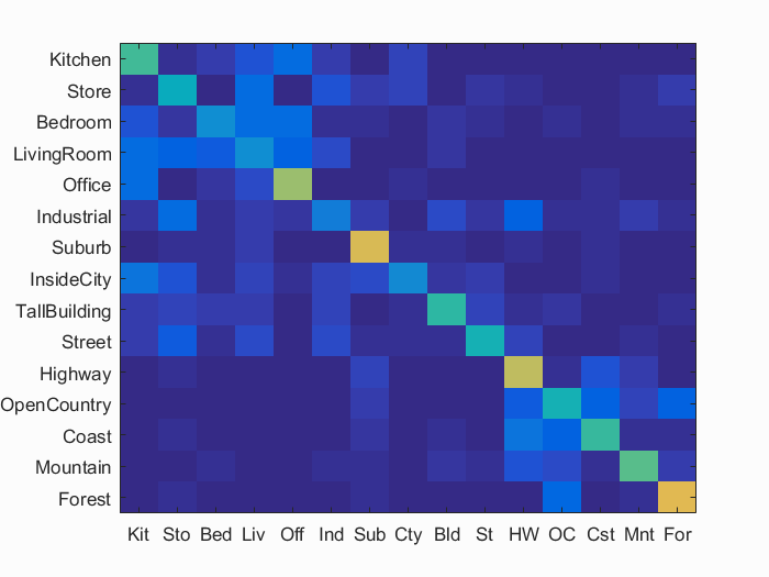Using the bags of SIFT features with the following parameters and KNN with K = 4, we can classify the testing images and achieve 49.0% accuracy.

vocab_size = 200;
in build_vocabulary.m: stepsize = 12, random_samples = 500, step = 8;
in get_bags_of_sifts.m: stepsize =6, random_samples = 1000, step = 4;

3. Bags of SIFT + 1 vs All Linear SVM

At last, 1 vs All Linear SVM is implemented to train and classify the images. 15 1-vs-all SVMs are trained to classify 'forest' vs 'non-forest', 'kitchen' vs 'non-kitchen', etc. For each testing image, 15 SVMs provide 15 real values which are between [-1, 1]. The maximum number among the 15 would define the category of this testing image. There is only one parameter lambda in this classifier. The optimum value actually varies based on the bags of feature representation. It is usually between 1e-5 and 1e-4. The one in the result is 4e-6. With bags of SIFT features and SVM classifier in the following set of parameters, the accuracy is 60.5%. And the total computational time is within 560s.

vocab_size = 200;
lambda = 4e-6;
in build_vocabulary.m: stepsize = 12, random_samples = 500, step = 8;
in get_bags_of_sifts.m: stepsize =6, random_samples = 1000, step = 4;

4. Extra credit/Graduate credit

1. 3 pts: Experiment with many different vocabulary sizes and report performance.

Suppose the visual words are well-sampled when building the vocabulary, then the number of clusters, i.e. vocab_size, would directly change the dimension of the feature vector for each image and thus have a big influence on the classifying result later on. Here we set all the parameters fixed and vary the vocab_size. The classifying accuracy varies. Note that, for each vocabulary size, the visual word vocabulary needs to be built individually. If the size is too small, then the images cannot be well-described and thus cannot be separated/classified. If the size is too large, then it is likely that the classifier ends up with overfitting. The result shown below meets the prediction.

in build_vocabulary.m: stepsize = 12, random_samples = 500, step = 8;
in get_bags_of_sifts.m: stepsize = 6, random_samples = 1000, step = 4;
lambda = 1e-5; 

Table 1 Accuracy of different vocabulary size.

vocab_size	10	20	50	100	200	400
Accuracy	47.2%	52.5%	58.8%	59.0%	60.5%	50.4%

1. 3 pts: Experiment with features at multiple scales.

In proj4extra, set FEATURE = 'bag of sift pyramid', and adjust the parameter pyramid between 1, 2 and 3, which represents rescale the image to 0.5, 0.25 and 0.125 of the original image size respectively. For each level of pyramid, we need to build the vocabulary correspondingly. The vocab_size = 200 is consistent throughout this comparison. For small scaled images, the step and step_size must be small enough to extract enough number of features. The parameters are set in the following rule so that there are enough sampled features in higher pyramid. The result is shown in Fig. 4.2 and Table 2. As the pyramid goes higher, a lot of information is losing thus the accuracy drops. However, even at 3 level pyramid, it could still achieve almost 40% accuracy, meaning that for down-sampled images, recognition can still be done at good rates.

vocab_size 200;
in build_vocabulary.m: stepsize = 12/pyramid_level, random_samples = 500, step = ceil(8/(2^pyramid_level));
in get_bags_of_sifts.m: stepsize = 6/pyramid_level, random_samples = 1000, step = ceil(8/(2^pyramid_level));
lambda = 1e-5; 

Table 2 Accuracy of different pyramid level.

Pyramid Level	0	1	2	3
Accuracy	60.5%	50.1%	49.1%	39.1%

1. 3 pts: Use "soft assignment" to assign visual words to histogram bins. Each visual word will cast a distance-weighted vote to multiple bins.

This is implemented in get_bags_of_sifts_soft.m and called from proj4extra. For each image, the sampled SIFT features have a distance matrix containing distances to each cluster center. The basic implementation was to select the closest cluster center for each SIFT feature and vote to the corresponding histogram bin. Here the 'soft assignment' is applied. Each SIFT feature votes to the nearest K bins based on the distance to the cluster centers. The closer, the more votes. The voted vectors in each image are summed and then normalized. There is one parameter nearestK to tune. When choosing it to be 30, the accuracy reaches to 70.1% (9.6% increases). The whole computation is done within 530s.

in build_vocabulary.m: stepsize = 12, random_samples = 500, step = 8;
in get_bags_of_sifts.m: stepsize = 6, random_samples = 1000, step = 4;
lambda = 1e-5; 

1. 3 pts: Use cross-validation to measure performance rather than the fixed test / train split provided by the starter code.

This implementation is in proj4cross.m. Instead of taking all the training and testing images, I extract 300 random number of training image and 300 random number of testing image, and do the iteration for 5 times using 'soft assignment' method. The accuracy is with mean = 57.46% and standard deviation = 0.024552.

Table 3 Accuracy for 5 runs.

# of runs	1	2	3	4	5
Accuracy	59.7%	59.0%	55.7%	57.7%	54.3%

1. 3 pts: Add a validation set to your training process to tune learning parameters.

This implementation is in svm_classify_with_validation.m. The lambda value for training each 1-vs-all SVM could vary. To find out the optimal lambda for each SVM, a validation set is randomly extracted from the training data. The rest of the training data is used to train each SVM. Then the learned SVM classifies the validation set and compare the classified result with the training label. The number of different labels is marked for different lambda. Then the lambda is chosen to provide least number of wrong classifying results. The same process is done for all the 15 SVMs to find the best lambda. During one experiment, the accuracy increases from 53.5% to 56.4%. However, due to the number of training data set is small, the improvement is not obvious and sometimes the accuracy drops due to overfitting.

1. 5 pts: Add additional gist descriptors and have the classifier consider them all.

Gist feature is used as an additional feature to build an additional visual vocabulary with 15 cluster center. For each training/testing image, the Gist feature is extracted as a 512 dimensional vector and its distances to all cluster centers is the feature vector. Thus, combining with the SIFT feature vector, each image would have 200+15 = 215 dimensional feature to train and test. The SVMs classifier is also adapted for this change. PCA is first done on the first 200 dimensional vector, and then the first 150 principle components are used to reduce the representation. Combine the 15 dimension GIST feature with the 150 dimensional reduced feature. Then the SVMs are trained and classified based on the 165 dimensional vectors. There is also a weight parameter 0.9 on the GIST feature. In this implementation, the accuracy reaches to 68.7% (8.2% increases).

Scene classification results : Best Results

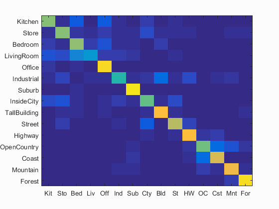
Accuracy (mean of diagonal of confusion matrix) is 0.701

Category name	Accuracy	Sample training images		Sample true positives		False positives with true label		False negatives with wrong predicted label
Kitchen	0.610		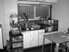			Industrial	LivingRoom	Bedroom	Bedroom
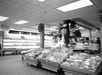
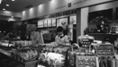
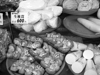
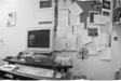
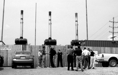
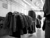
Store	0.620		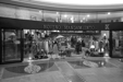			LivingRoom	Street	Mountain	Office
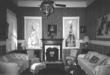
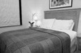
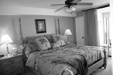
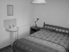
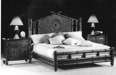
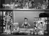
Bedroom	0.640					LivingRoom	Store	InsideCity	TallBuilding
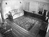
LivingRoom	0.320					Highway	Bedroom	Kitchen	Bedroom
Office	0.910		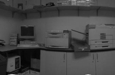			Store	Bedroom	Kitchen	InsideCity
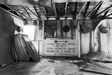
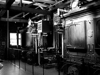
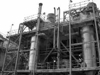
Industrial	0.470		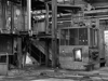			Store	Mountain	Office	Store
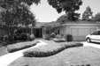
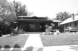
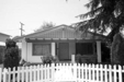
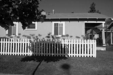
Suburb	0.940		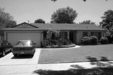			Bedroom	Coast	Bedroom	Bedroom
InsideCity	0.570					Industrial	Mountain	Bedroom	Store
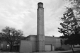
TallBuilding	0.830					Industrial	Industrial	Street	Coast
Street	0.690					Store	InsideCity	InsideCity	TallBuilding
Highway	0.830					Store	Street	LivingRoom	Street
OpenCountry	0.590					Mountain	Coast	Bedroom	Coast
Coast	0.750					OpenCountry	Highway	OpenCountry	OpenCountry
Mountain	0.810					Coast	LivingRoom	Suburb	OpenCountry
Forest	0.930					Store	Mountain	Street	Mountain
Category name	Accuracy	Sample training images		Sample true positives		False positives with true label		False negatives with wrong predicted label