Yishan Chen

Tiny Images Representation

The "tiny image" feature is one of the simplest possible image representations. The steps of this algorithm are very simple:

1. Resizes each image to a small, fixed resolution (16x16 as recommanded).
2. Make the tiny image to have zero mean.
3. Repeat until all images are processed.

Nearest Neighbor Classifier

The nearest neighbor classifier simply finds the "nearest" training example and assigns the test case the label of that nearest training example when tasked with classifying a test feature into a particular category.

After reading training and testing features, the distance between them can be calculated by the vl_alldist2() function in VLFeat library:

dist(j) = vl_alldist2(train',test');

For each testing image, iterate through all training images and calculate the distances between them. Find the minimum distance and label the testing image with the category of the corresponding training image:

[mind,ind] = min(dist);
predicted_categories(i,1) = train_labels(ind);

Bag of SIFT Representation

There are two steps to build the bags of quantized SIFT features: establish a vocabulary of visual words and represent our training and testing images as histograms of visual words.

Build Vocabulary

We will form this vocabulary by sampling many local features from training set and then clustering them with kmeans.

First, read images and use vl_dsift() function to extracts a dense set of SIFT features from images. I use the "fast" parameter and extracts a SIFT descriptor each 5 pixels to make the program faster.

[locations, SIFT_features] = vl_dsift(single(img),'fast', 'Step', 5);

After that, randomly select 100 features from the sift features of each images and then collect features of all pictures to form a matrix X of sampled SIFT features. Then, use VL_KMEANS(X, NUMCENTERS) to cluster the columns of the matrix X in NUMCENTERS centers C using k-means. The vocab matrix is formed by transposing the centers calculated by k-means:

[centers, assignments] = vl_kmeans(X, vocab_size);
vocab = centers';

Implement Histogram

With the vocabulary of visual words, training and testing images can be represented as histograms. The steps of this algorithm are listed as follows:

1. Load the built vocabulary matrix.
2. Load testing images and extract SIFT descriptors.
3. For each image, find the nearest neighbor kmeans centroid for every SIFT feature. The feature is tagged to the cluster with the closest center and add one to the index of the respective clusters in the histogram.
4. Normalize the histogram so that image size does not dramatically change the bag of feature magnitude.

Linear SVM Classifier

The task of this part is to train a linear SVM for every category and then use the learned linear classifiers to predict the category of every test image. Every test feature will be evaluated with all 15 SVMs and the SVM with the highest confidence will be the predicted label. Confidence, or distance from the margin, is W*X + B where '*' is the inner product or dot product and W and B are the learned hyperplane parameters.

While training, a matrix of binary labels (-1 or 1) are created from the comparison of the category name for that instance and the training labels for each of the 15 categories. Use the function vl_svmtrain(features, labels, LAMBDA) to train a linear Support Vector Machine (SVM) from the data features and the labels. LAMBDA regularizes the linear classifier by encouraging W to be of small magnitude and is very important in the function. In my program, LAMBDA is set to be 0.00001:

for i = 1:num_categories

    bin_labels = double(strcmp(categories(i),train_labels));
    bin_labels(bin_labels==0) = -1;

    [W(i,:) B(i,:)] = vl_svmtrain(train_image_feats', bin_labels', LAMBDA);
end

After trainiing, the confidence of features for each images are computed by W*X + B:

for j = 1:num_categories
	W2 = W(j,:)';
	confidence(j) = dot(W2, feat') + B(j,:);
end

Find the maximum confidence and label the testing image with the category of the corresponding training image.

[maxc,maxid] = max(confidence);
predicted_categories(i,1) = categories(maxid); 

Extra Credit for Feature Representation: Gist Descriptors

The gist descriptor is based on a very low dimensional representation of real world scenes that bypasses the segmentation and the processing of individual objects or regions. I use the function LMgist given by Aude Oliva and Antonio Torralba to compute gist features:

img = imread(char(image_paths(i)));  
[gist(i,:),param] = LMgist(img, '', param);

The image is first divided into a grid of 4x4 cells. The number of orientations per scale (from HF to LF) is set to be [8 8 8 8]. When computing image similarities, image size needs to be normalized before computing the GIST descriptor. In my program, the images are resized to be 256x256.

Extra Credit for Experimental Design

I implement cross-validation to measure performance and experiment with many different vocabulary sizes. The detailed analysis of these two parts are in the results chapter.

Results

Tiny Images Representation with Nearest Neighbour Classification

The tiny image representation and nearest neighbor classifier gets a very low accuracy as 20.1% over a short time of 20.95s on the 15 scene database. For comparison, chance performance is ~7%.

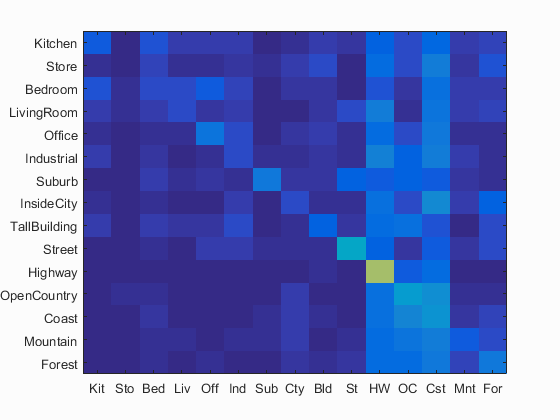
Accuracy is 0.201. Click for Detailed Results

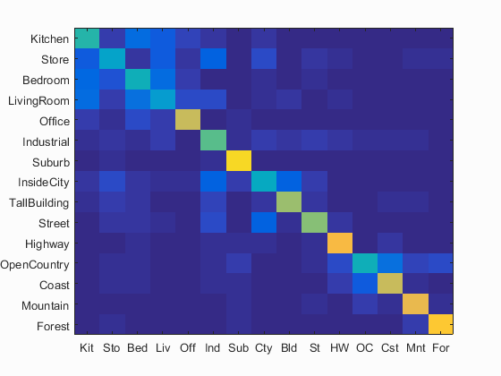
Bag of SIFT with Nearest Neighbour Classification

Bag of SIFT representation with a nearest neighbor classifier works much better than tiny images. I set the vocabulary size to be 200 and get an accuracy as 51.3%. However, it takes 3441s to get the result, which is much longer than tiny images.

Accuracy is 0.513. Click for Detailed Results

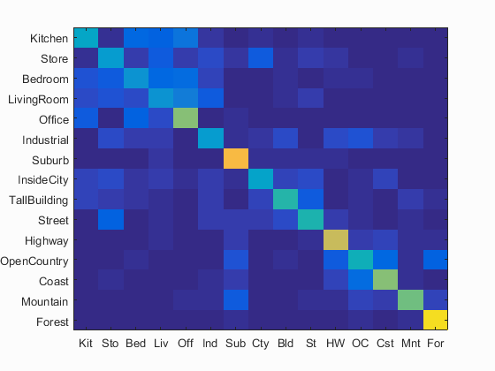
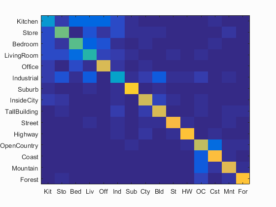
Bag of SIFT with Linear SVM

Bag of SIFT representation with Linear SVM works even better than bag of SIFT representation with a nearest neighbor classifier. I set the vocabulary size to be 200, LAMBDA to be 0.00001 and get an accuracy as 60.8%. It takes 3612s to get the result, even longer than bag of SIFT representation with a nearest neighbor classifier.

Accuracy is 0.608. Click for Detailed Results

GIST with Nearest Neighbour Classification and Linear SVM

GIST descriptor has higher accuracy than SIFT in both nearest neighbour classification and linear SVM. Meanwhile, it is much faster. It takes 724.3s to get results of 56.1% accuracy by nearest neighbour classification and 725.3s to get results of 68.5% accuracy by linear SVM.

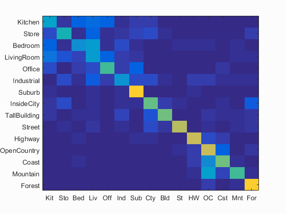
Accuracy is 0.561 by nearest neighbour classification. Click for Detailed Results
Accuracy is 0.685 by linear SVM. Click for Detailed Results

Cross Validation

To get a more accurate performance measure, I did a cross validation by randomly picking 100 training and 100 testing images for each iteration. I iterate 10 times for the the tiny image representation and nearest neighbor classifier algorithm (since it is fast). The followings are the results:

	1	2	3	4	5	6	7	8	9	10	Average	Standard Deviation
Accuracy	0.199	0.205	0.209	0.216	0.211	0.207	0.191	0.207	0.207	0.205	0.2057	0.006767
Results	Click	Click	Click	Click	Click	Click	Click	Click	Click	Click

The accuracy of the tiny image representation and nearest neighbor classifier algorithm are quite stable and change little among the iteration.

Experiment with Different Vocabulary Sizes

I experiment with different vocabulary sizes as 10, 20, 50, 100, 200, 400 of bag of SIFT representation and test performance by nearest neighbour classification and linear SVM. The followings are the results of my experiment:

Vocabulary Size	Time		Accuracy		Results
	Nearest Neighbour	linear SVM	Nearest Neighbour	linear SVM	Nearest Neighbour	linear SVM
10	328s	240s	0.373	0.411	Click	Click
20	437s	434s	0.431	0.505	Click	Click
50	942s	940s	0.487	0.563	Click	Click
100	1787s	1786s	0.500	0.589	Click	Click
200	3441s	3612s	0.513	0.608	Click	Click
400	7148s	6832s	0.515	0.654	Click	Click

From the table, we can draw following conclusions:

1. For all vocabulary sizes, linear SVM always perform better than nearest neighbour classification.
2. When vocabulary size increased, the computing time increased as well.
3. When vocabulary size increased, the accuracy of results increased as well.
4. The computing time increases in proportion to vocabulary size.
5. The accuracy of results increases fast at the beginning and then become slower.

From the table, we can find that the accuracy of bag of SIFT representation with a nearest neighbor classifier increases very slow when the vocabulary size is bigger than 100, while the computing time increases much faster. For linear SVM, the accuracy is still increasing when the vocabulary size is bigger than 100, but it is slower than before.

Therefore, in order to get accurate results and control the time cost of the program, setting the vocabulary size to be 200 will be a good choice.

Since the program spends long time to computing results, I'll use my computer to do something else when running the code. As a result, the time may not be very precise. In some cases nearest neighbour classification spends more time, but in other cases linear SVM spends more time.

Then I try to save the matrix of training and testing features of the bag of SIFT part, and load them before classification. As a result, I find that the time cost of nearest neighbour classification and linear SVM is quite similar and is much smaller than the time needed for computing bag of SIFT features. Therefore, in order to get accurate results and control the time cost of the program, using linear SVM will be a better choice.