Project 4 Scene Recognition with Bag of Words

Tiny images representation

The "tiny image" feature, inspired by the work of the same name by Torralba, Fergus, and Freeman, is one of the simplest possible image representations. One simply resizes each image to a small, fixed resolution. It works slightly better if the tiny image is made to have zero mean and unit length. This is not a particularly good representation, because it discards all of the high frequency image content and is not especially invariant to spatial or brightness shifts. We will not worry about alignment for this project. We are using tiny images simply as a baseline.

To build a tiny image feature, simply resize the original image to a very small square resolution, e.g. 16x16. You can either resize the images to square while ignoring their aspect ratio or you can crop the center square portion out of each image. Making the tiny images zero mean and unit length (normalizing them) will increase performance modestly.


image = imresize(image, [d, d]);
image = reshape(image, [1, d * d]);
image = image - mean(image);
image_normalized = image / norm(image);

Bag of SIFT representation

Because of the alignment problem of tiny images representation, it is time to move on to a more sophisticated image representation -- bags of quantized SIFT features.Before we can represent our training and testing images as bag of feature histograms, we first need to establish a vocabulary of visual words.This vocabulary is formed by sampling many local features from the training set and then clustering them with kmeans.


nImage = size(image_paths, 1);
nEachImageFeature = ceil(vocab_size * 50 / nImage);
ImageFeatures = zeros(128, nEachImageFeature * nImage);
for i = 1 : nImage
    fprintf('building vocabulary from image %d\n', i);
    image_name = image_paths{ i };
    image = im2single(imread(image_name));
    [~, SIFT_features] = vl_dsift(image, 'step', 10, 'fast');
    index = randsample(size(SIFT_features, 2), nEachImageFeature);
    ImageFeatures(:, (i - 1) * nEachImageFeature + 1 : i * nEachImageFeature) = SIFT_features(:, index);
end
[centers, ~] = vl_kmeans(single(ImageFeatures), vocab_size);
vocab = centers';

Now we are ready to represent our training and testing images as histograms of visual words. For each image we will densely sample many SIFT descriptors. Instead of storing hundreds of SIFT descriptors, we simply count how many SIFT descriptors fall into each cluster in our visual word vocabulary. This is done by finding the nearest neighbor kmeans centroid for every SIFT feature.


load('vocab.mat')
vocab_size = size(vocab, 1);
nImage = size(image_paths, 1);
image_feats = zeros(nImage, vocab_size);
for i = 1 : nImage
   fprintf('get bags of sift from image %d\n', i);
   image_name = image_paths{ i };
   image = im2single(imread(image_name));
   [~, SIFT_features] = vl_dsift(image, 'step', 10, 'fast');
   D = vl_alldist2(vocab', single(SIFT_features));
   for j = 1 : size(SIFT_features, 2)
       [~, index] = min(D(:, j));
       image_feats(i, index) = image_feats(i, index) + 1;
   end
   image_feats(i, :) = image_feats(i, :) / norm(image_feats(i, :));
end

Nearest Neighbor Classifier

When tasked with classifying a test feature into a particular category, one simply finds the "nearest" training example (L2 distance is a sufficient metric) and assigns the test case the label of that nearest training example. The nearest neighbor classifier has many desirable features -- it requires no training, it can learn arbitrarily complex decision boundaries, and it trivially supports multiclass problems.

However, it's quite vulnerable to training noise, though, which can be alleviated by voting based on the K nearest neighbors. Nearest neighbor classifiers also suffer as the feature dimensionality increases, because the classifier has no mechanism to learn which dimensions are irrelevant for the decision

To implement voting from K-nearest neighbor, I used map container in matlab.


D = vl_alldist2(train_image_feats', test_image_feats');
for i = 1: nTestImage
    [~, index] = sort(D(:, i));
    mapObj = containers.Map;
    for j = 1 : k
        if isKey(mapObj, train_labels{ index(j) })
            mapObj(train_labels{ index(j) }) = mapObj(train_labels{ index(j) }) + 1;
        else
            mapObj(train_labels{ index(j) }) = 1;
        end
    end
    keySet = keys(mapObj)';
    valueSet = values(mapObj)';
    [~, keyIndex] = sortrows(valueSet, [-1]);
    predicted_categories{ i } = keySet{ keyIndex(1) };
end

1-vs-all linear SVM

Linear classifiers are one of the simplest possible learning models. The feature space is partitioned by a learned hyperplane and test cases are categorized based on which side of that hyperplane they fall on.

However, linear classifiers are inherently binary and we have a 15-way classification problem. To decide which of 15 categories a test case belongs to, we will train 15 binary, 1-vs-all SVMs. 1-vs-all means that each classifier will be trained to recognize 'forest' vs 'non-forest', 'kitchen' vs 'non-kitchen', etc.


categories = unique(train_labels);
num_categories = length(categories);
nTrainImage = size(train_image_feats, 1);
nFeatures = size(train_image_feats, 2);
lambda = 0.5;
W = zeros(num_categories, nFeatures); B = zeros(num_categories, 1);
for i = 1 : num_categories
    labels = -1 * ones(nTrainImage, 1);
    matching_indices = strcmp(categories{i}, train_labels);
    labels(matching_indices) = 1;
    [w, b] = vl_svmtrain(train_image_feats', labels, lambda);
    W(i, :) = w'; B(i) = b;
end

All 15 classifiers will be evaluated on each test case and the classifier which is most confidently positive "wins". E.g. if the 'kitchen' classifier returns a score of -0.2 (where 0 is on the decision boundary), and the 'forest' classifier returns a score of -0.3, and all of the other classifiers are even more negative, the test case would be classified as a kitchen even though none of the classifiers put the test case on the positive side of the decision boundary.


predicted_categories = cell(nTestImage, 1);
for i = 1 : nTestImage
	scores = zeros(num_categories, 1);
	for j = 1 : num_categories
		scores(j) = W(j, :) * test_image_feats(i, :)' + B(j);
	end
	[~, index] = max(scores);
	predicted_categories{ i } = categories{ index };
end

Result

Tiny images representation and nearest neighbor classifier

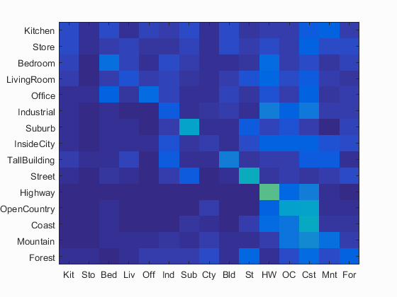
Accuracy (mean of diagonal of confusion matrix) is 0.224

Bag of SIFT representation and nearest neighbor classifier

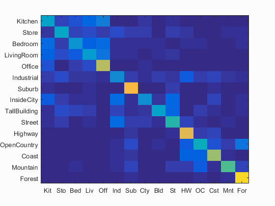
Accuracy (mean of diagonal of confusion matrix) is 0.508

Bag of SIFT representation and linear SVM classifier

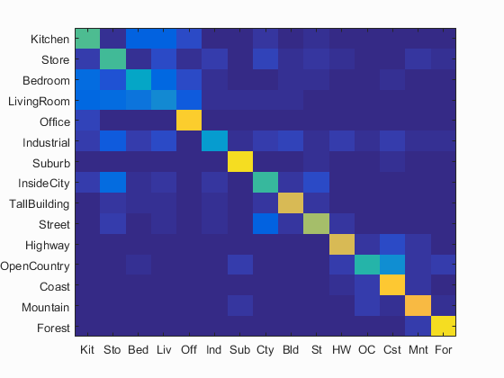
Accuracy (mean of diagonal of confusion matrix) is 0.643

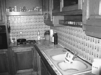
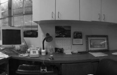
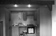
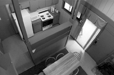
Scene classification results of Bag of SIFT representation and linear SVM classifier

Category name	Accuracy	Sample training images	Sample true positives	False positives with true label		False negatives with wrong predicted label
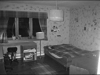
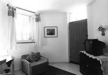
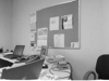
Kitchen	0.540			Bedroom	Office	Bedroom	Mountain
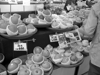
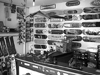
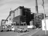
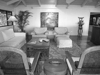
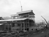
Store	0.530		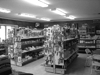	LivingRoom	InsideCity	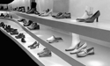Mountain	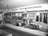Kitchen
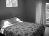
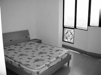
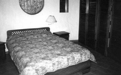
Bedroom	0.380		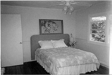	Kitchen	LivingRoom	Kitchen	Office
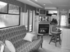
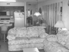
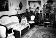
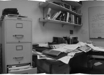
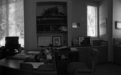
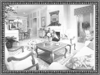
LivingRoom	0.270		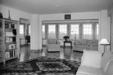	Industrial	Bedroom	Bedroom	Store
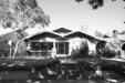
Office	0.890		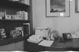	Bedroom	LivingRoom	TallBuilding	Kitchen
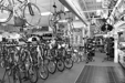
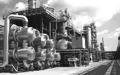
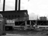
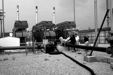
Industrial	0.340		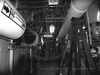	Suburb	TallBuilding	InsideCity	LivingRoom
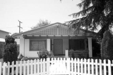
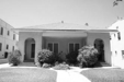
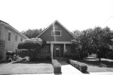
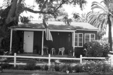
Suburb	0.930		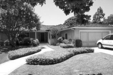	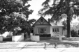Industrial	Mountain	Mountain	Store
InsideCity	0.510			Street	LivingRoom	Store	TallBuilding
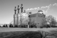
TallBuilding	0.750			Industrial	Office	Suburb	Industrial
Street	0.670			InsideCity	Store	Store	InsideCity
Highway	0.760			Industrial	Store	Mountain	Coast
OpenCountry	0.470			Mountain	Highway	Coast	Coast
Coast	0.860			OpenCountry	Mountain	OpenCountry	OpenCountry
Mountain	0.820			Street	Coast	Industrial	OpenCountry
Forest	0.930			OpenCountry	Mountain	Mountain	Mountain
Category name	Accuracy	Sample training images	Sample true positives	False positives with true label		False negatives with wrong predicted label

From confusion matrix and results of Bag of SIFT with linear SVM, we can see the algorithm cannot distinguish Kitchen, Store, Bedroom, Living Room very well.

It seems these rooms are difficult to distinguish because they sometimes share the furniture of similar shape. For example, most bedroom has a bed, but possibly the sofa in the living room looks very similar to a bed. Tables and chairs may also play an important role here.

Extra Point

1. Add additional, complementary features

I choose to add a gist descriptor and make linear SVM to consider it with bag of words. I extract all the gist descriptor from train image and test image (one descriptor per image) and use linear SVM to score them.

The problem is how we combine the two scores, one of gist and the other of bag of SIFTs. I decide to respectively sort the scores and get the rank of each scene. Then I add the two ranks of each scene. For example, if scene A rank 1st in term of gist and 2nd in term of bags of SIFTs, then it's total rank is 3. Those with least total ranks will be judged as the optimum.


[~, index1] = sort(scores1, 'descend'); Inverse_index1(index1) = 1 : num_categories;
[~, index2] = sort(scores2, 'descend'); Inverse_index2(index2) = 1 : num_categories;
[~, index] = min(Inverse_index1 + Inverse_index2);
predicted_categories{ i } = categories{ index };

Bag of SIFT representation with Gist Discriptor and linear SVM classifier

Accuracy (mean of diagonal of confusion matrix) is 0.667

This method can improve the accurcy from 0.643 to 0.667

2. Train the SVM with Gaussian kernel

I use Olivier Chapelle's MATLAB code for primal SVM

The Guassian kernel matrix is calculated as


nsq = sum(train_image_feats .^ 2, 2);
K = bsxfun(@minus,nsq,(2 * train_image_feats) * train_image_feats.');
K = bsxfun(@plus, nsq.', K);
K = exp(-K);

Bag of SIFT representation and Gaussian SVM classifier

Accuracy (mean of diagonal of confusion matrix) is 0.663

This method can improve the accurcy from 0.643 to 0.663

3. Experiment with many different vocabulary sizes

vocabulary sizes	accuracy
10	0.417
20	0.493
50	0.571
100	0.621
100	0.643
400	0.637
1000	0.648

References

[1] Aude Oliva, Antonio Torralba. International Journal of Computer Vision, Vol. 42(3): 145-175, 2001

[2] Olivier Chapelle. Training a Support Vector Machine in the Primal, in press

Yidong Liu

Project 4 Scene Recognition with Bag of Words