Project 4 Scene Recognition with Bag of Words
Step 1 - File edited: get_tiny_images.m
In this file, I rescaled all the images to be 16 by 16 and ignore their aspect ratio.
Step 2 - File edited: nearest_neighbor_classify.m
In this file, I used default distance measure, L2, to find the nearest training examples and assign the test case with the training label of that match.
When tiny images and nearest neighbor classifer are used, I achieved the accuracy of 19.1%
Step 3 - File edited: build_vocabulary.m
This file is used to build the vocabulary database to construct the histogram during the later task. I collected 100 sift features from each image and tried step size of both 10 and 20. I finally decided to keep step size as 20 due to runtime concern. Since the step size in get_bags_of_sift.m is supposed to be smaller or equal to the step size of build_vocabulary.m, using 20 for build_vocabulary allows me to amplify the step size in get_bags_of_sift.m to reduce computations.
Step 4 - File edited: get_bags_of_sifts.m
This file helps us to construct the histogram that explains the features of the test images. Likewise, sift features are collected from each test images and compared against the vocabulary we built ealier. For each feature from test image, we find the closest feature match it has on the vacabulary and adds 1 to each bin. We normalize the histograms and return it. I chose step size of 10 in this file as it seems to give me the highest accuracy rate.
When bags of sifts and nearest neighbor classifer are used, I achieved accuracy of 52.9%.
categories = unique(train_labels);
num_categories = length(categories);
predicted_categories = cell(size(test_image_feats,1),1);
confidence_matrix = zeros(size(test_image_feats,1),num_categories);
for i=1:num_categories
    indices = strcmp(categories(i),train_labels);
    train_binary = zeros(length(indices),1);
    for l=1:length(indices)
        if indices(l) == 0
            train_binary(l) = -1;
        else
            train_binary(l) = 1;
        end
    end
    [W,B] = vl_svmtrain(train_image_feats', train_binary, 0.0003);
    for j=1:size(test_image_feats,1)
        confidence = dot(W,(test_image_feats(j,:))') + B;
        confidence_matrix(j,i) = confidence;
    end
end
Above is part of the code from the file. For each unique category, i selected pictures of that category from training samples and set their label to 1. Then I constructed SVM for each category and calculate the score of each test picture using that SVM. Eventually, each test image will get number of scores equal to the number of categories and select the category that seems to most likely fit the test image. For the choice of lambda, I tried multiple numbers, and finally set the lambda = 0.0003 as it renders the highest accuracy rate.
Results in a table
| lambda | Feature selection | Classifier | Accuracy | Runtime |
|---|---|---|---|---|
| Tiny images | Nearest Neighbor | 19.1 | pretty short | |
| Bags of SIFT (vocab step = 10,bags of sift step = 5) | Nearest Neighbor | 53.3 | 17 mins | |
| Bags of SIFT (vocab step = 10,bags of sift step = 10) | Nearest Neighbor | 50.8 | 12 mins | |
| Bags of SIFT (vocab step = 20,bags of sift step = 10) | Nearest Neighbor | 52.9 | 8 mins | |
| 0.00001 | Bags of SIFT (vocab step = 10,bags of sift step = 5) | SVM | 66.1 | 12 mins |
| 0.0001 | Bags of SIFT (vocab step = 10,bags of sift step = 5) | SVM | 68.3 | 12 mins |
| 0.001 | Bags of SIFT (vocab step = 10,bags of sift step = 5) | SVM | 60.5 | 12 mins |
| 0.0005 | Bags of SIFT (vocab step = 10,bags of sift step = 5) | SVM | 65.1 | 12 mins |
| 0.0001 | Bags of SIFT (vocab step = 20,bags of sift step = 10) | SVM | 62.7 | 8 mins |
| 0.0005 | Bags of SIFT (vocab step = 20,bags of sift step = 10) | SVM | 61.7 | 8 mins |
| 0.0003 | Bags of SIFT (vocab step = 20,bags of sift step = 10) | SVM | 63.3 | 8 mins |
The selection of parameters seem to affect the prediction accuracy a lot in this project. As we can tell from the table, the smaller step size for bags of sifts, the more accurate the prediction gets, because more features are extracted from each test image. This comes with the tradeoff of runtime, as more feature extraction will result in more computation and therefore lengthen the runtime. In order to make all the pipelines work under 10 minutes mark, I had to sacrifice a little accuracy for speed and choose the step size of bag of sifts to be 10.
Also, the SVM is very sensitive to lambda value. SVM tends to maximize the margin between classes and for nonseperable problems, the miss-classification constraint needs to be relaxed through setting up the regularization. A smaller lamdba value will allow more mis-classifications. In our case, it seems the best range is between 0.0001 - 0.0003 to have the highest accuracy.
Scene classification results visualization
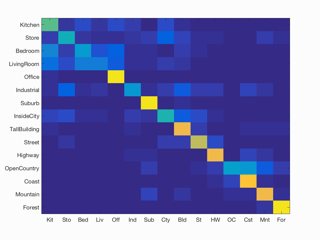
Accuracy (mean of diagonal of confusion matrix) is 0.631
| Category name | Accuracy | Sample training images | Sample true positives | False positives with true label | False negatives with wrong predicted label | ||||
|---|---|---|---|---|---|---|---|---|---|
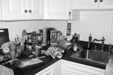
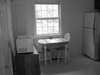
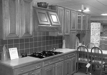
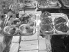
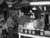
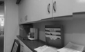
| Kitchen | 0.560 | 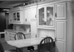 |
 |
 |
 |
 Bedroom |
 Industrial |
 TallBuilding |
 Bedroom |
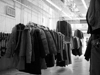
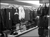
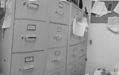
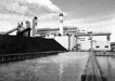
| Store | 0.430 |  |
 |
 |
 |
 Industrial |
 Street |
 TallBuilding |
 TallBuilding |
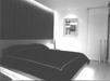
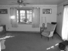
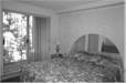
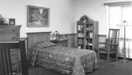
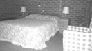
| Bedroom | 0.340 | 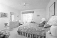 |
 |
 |
 |
 LivingRoom |
 Industrial |
 Street |
 Office |
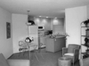
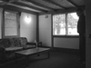
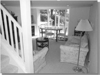
| LivingRoom | 0.220 | 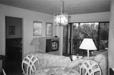 |
 |
 |
 |
 Store |
 Store |
 Office |
 Kitchen |
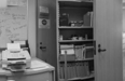
| Office | 0.940 |  |
 |
 |
 |
 Kitchen |
 LivingRoom |
 Kitchen |
 Kitchen |
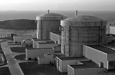
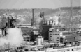
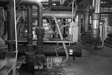
| Industrial | 0.320 | 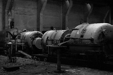 |
 |
 |
 |
 Bedroom |
 Street |
 Coast |
 Store |
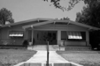
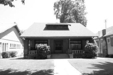
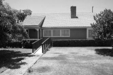
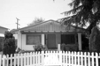
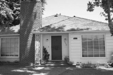
| Suburb | 0.940 | 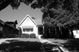 |
 |
 |
 |
 Bedroom |
 OpenCountry |
 Store |
 LivingRoom |
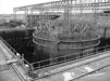
| InsideCity | 0.460 |  |
 |
 |
 |
 Kitchen |
 Industrial |
 Bedroom |
 Industrial |
| TallBuilding | 0.800 |  |
 |
 |
 |
 Store |
 Bedroom |
 Street |
 Street |
| Street | 0.710 |  |
 |
 |
 |
 InsideCity |
 Kitchen |
 Mountain |
 TallBuilding |
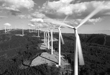
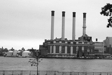
| Highway | 0.800 |  |
 |
 |
 |
 OpenCountry |
 Store |
 Coast |
 Suburb |
| OpenCountry | 0.350 |  |
 |
 |
 |
 Mountain |
 Coast |
 Coast |
 Street |
| Coast | 0.850 |  |
 |
 |
 |
 OpenCountry |
 OpenCountry |
 OpenCountry |
 OpenCountry |
| Mountain | 0.800 |  |
 |
 |
 |
 OpenCountry |
 Coast |
 TallBuilding |
 TallBuilding |
| Forest | 0.940 |  |
 |
 |
 |
 TallBuilding |
 Store |
 Industrial |
 Street |
| Category name | Accuracy | Sample training images | Sample true positives | False positives with true label | False negatives with wrong predicted label | ||||