Project 4: Scene recognition with bag of words
The objective of the project Scene recognition with bag of words is to recognize a scene using tiny images and bags of local features and perform classification with nearest neighbor and support vector machine method. The best accuracy ever achieved by this program is 68.5% recognition accuracy.
Methodology
1. Tiny image representation with nearest neighbor classifier
Using the 16*16 tiny image representation and training the data with a nearest neighbor classifier, the overall accuracy of the system reaches 22.5%.
Scene classification results visualization
Accuracy (mean of diagonal of confusion matrix) is 0.225
| Category name | Accuracy | Sample training images | Sample true positives | False positives with true label | False negatives with wrong predicted label | ||||
|---|---|---|---|---|---|---|---|---|---|
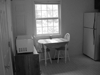
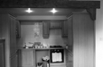
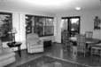
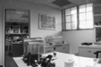
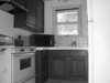
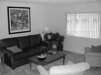
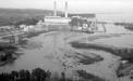
| Kitchen | 0.080 |  |
 |
 |
 |
 LivingRoom |
 Coast |
 Coast |
 Bedroom |
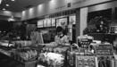
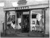
| Store | 0.020 | 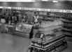 |
 |
 |
 |
 Forest |
 Forest |
 TallBuilding |
 InsideCity |
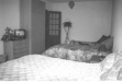
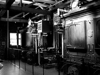
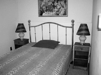
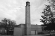
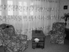
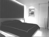
| Bedroom | 0.180 |  |
 |
 |
 |
 Industrial |
 Office |
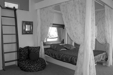 LivingRoom |
 Highway |
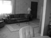
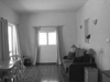
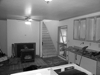
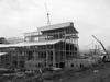
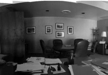
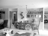
| LivingRoom | 0.100 | 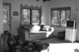 |
 |
 |
 |
 Coast |
 Bedroom |
 Mountain |
 Industrial |
| Office | 0.160 |  |
 |
 |
 |
 Forest |
 LivingRoom |
 Forest |
 Bedroom |
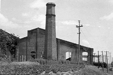
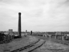
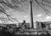
| Industrial | 0.130 |  |
 |
 |
 |
 Mountain |
 InsideCity |
 Mountain |
Bedroom |
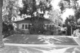
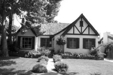
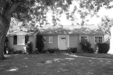
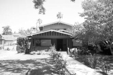
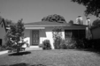
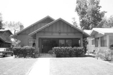
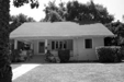
| Suburb | 0.370 |  |
 |
 |
 |
 Kitchen |
 Street |
 OpenCountry |
 Forest |
| InsideCity | 0.060 |  |
 |
 |
 |
 Kitchen |
 Bedroom |
 Forest |
 Highway |
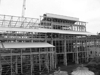
| TallBuilding | 0.230 |  |
 |
 |
 |
 Industrial |
 LivingRoom |
 Coast |
 InsideCity |
| Street | 0.420 |  |
 |
 |
 |
 Store |
 Suburb |
 Forest |
 Coast |
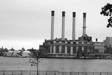
| Highway | 0.560 |  |
 |
 |
 |
 TallBuilding |
 LivingRoom |
 Coast |
 Mountain |
| OpenCountry | 0.350 |  |
 |
 |
 |
 Coast |
 Forest |
 Coast |
 Coast |
| Coast | 0.400 |  |
 |
 |
 |
 Office |
 Mountain |
 OpenCountry |
 InsideCity |
| Mountain | 0.180 |  |
 |
 |
 |
 InsideCity |
 Kitchen |
 Coast |
 Office |
| Forest | 0.130 |  |
 |
 |
 |
 Kitchen |
Store |
 Street |
 Street |
| Category name | Accuracy | Sample training images | Sample true positives | False positives with true label | False negatives with wrong predicted label | ||||
2. Bags of SIFT features with nearest neighbor classifier
Two steps are conducted in this part. First, a vocabulary of size 200 is built using the training data. 20 features are randomly obtained from each image, with k-means clustering method applied afterwards to obtain the 500 centers for the vocabulary. Next, 1000 features are obtained from each image to form the histogram for each training and testin image. The label of the testing image is assigned by its nearest neighbor image in the training set. The overall accuracy reaches 52.3%.
Scene classification results visualization
Accuracy (mean of diagonal of confusion matrix) is 0.523
| Category name | Accuracy | Sample training images | Sample true positives | False positives with true label | False negatives with wrong predicted label | ||||
|---|---|---|---|---|---|---|---|---|---|
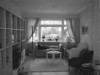
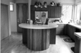
| Kitchen | 0.410 |  |
 |
 |
 |
 Bedroom |
 Street |
 InsideCity |
 InsideCity |
| Store | 0.400 |  |
 |
 |
 |
 LivingRoom |
 Industrial |
 LivingRoom |
 Bedroom |
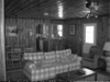
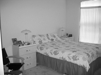
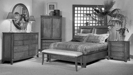
| Bedroom | 0.390 |  |
 |
 |
 |
 InsideCity |
 TallBuilding |
 Kitchen |
 TallBuilding |
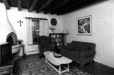
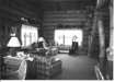
| LivingRoom | 0.240 |  |
 |
 |
 |
 TallBuilding |
 Suburb |
 Industrial |
 Office |
| Office | 0.710 |  |
 |
 |
 |
 Kitchen |
 Kitchen |
 LivingRoom |
 Kitchen |
| Industrial | 0.320 | 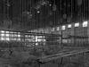 |
 |
 |
 |
 TallBuilding |
 InsideCity |
 Forest |
 InsideCity |
| Suburb | 0.760 |  |
 |
 |
 |
 Mountain |
 Store |
 Store |
 InsideCity |
| InsideCity | 0.360 |  |
 |
 |
 |
 Store |
 Industrial |
 Coast |
Industrial |
| TallBuilding | 0.460 |  |
 |
 |
 |
 Industrial |
 InsideCity |
 Suburb |
 Industrial |
| Street | 0.500 |  |
 |
 |
 |
 TallBuilding |
 InsideCity |
 LivingRoom |
 Store |
| Highway | 0.750 |  |
 |
 |
 |
 OpenCountry |
 Suburb |
 Coast |
 OpenCountry |
| OpenCountry | 0.450 |  |
 |
 |
 |
 Highway |
 Coast |
 Forest |
 Mountain |
| Coast | 0.620 |  |
 |
 |
 |
 OpenCountry |
 Highway |
 Suburb |
 Highway |
| Mountain | 0.520 |  |
 |
 |
 |
 Industrial |
 Bedroom |
 Street |
 Forest |
| Forest | 0.950 |  |
 |
 |
 |
 OpenCountry |
 Store |
 Mountain |
 Mountain |
| Category name | Accuracy | Sample training images | Sample true positives | False positives with true label | False negatives with wrong predicted label | ||||
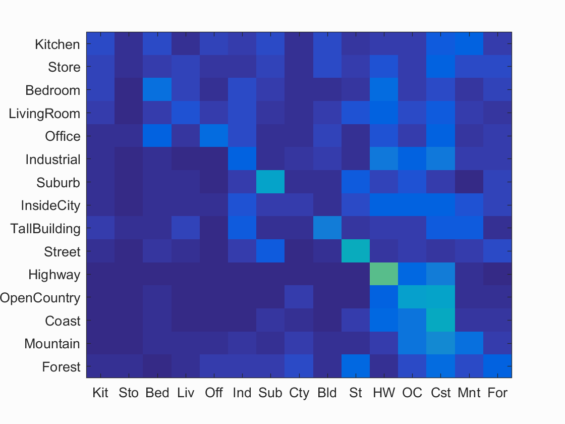
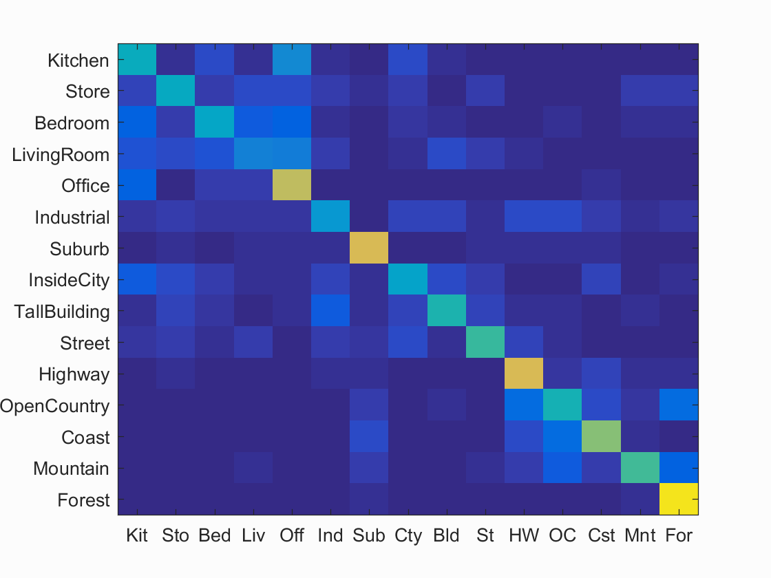
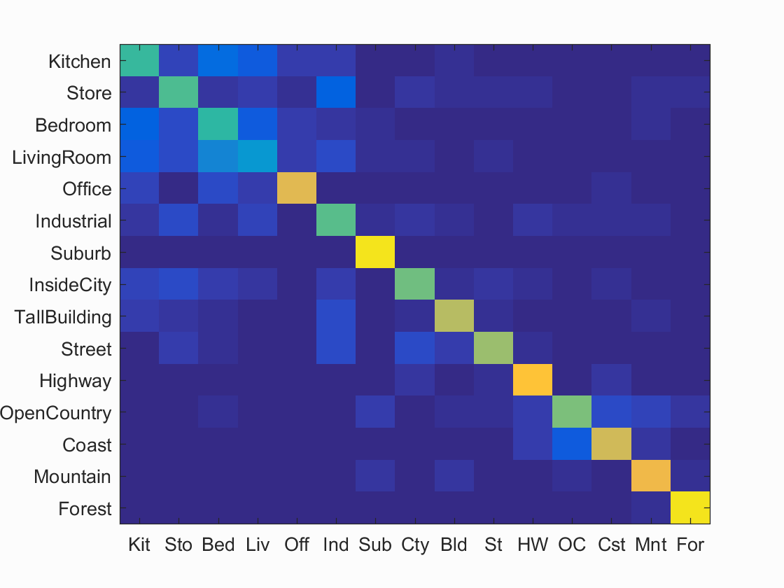
3. Bags of SIFT features with support vector machine
This part differes from part2 only by the classifier chosen. Instead of using nearest neighbor classifier, 15 support vector machine classifiers are used with one for each class. The algorithm reaches 63.1% accuracy.
Scene classification results visualization
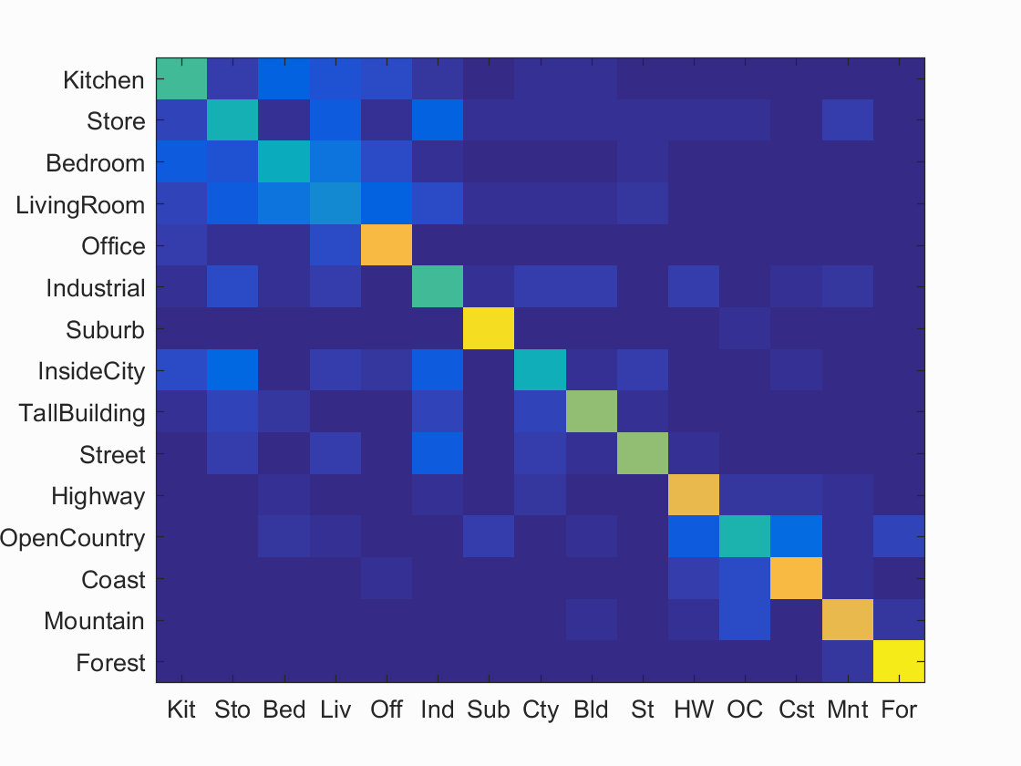
Accuracy (mean of diagonal of confusion matrix) is 0.631
| Category name | Accuracy | Sample training images | Sample true positives | False positives with true label | False negatives with wrong predicted label | ||||
|---|---|---|---|---|---|---|---|---|---|
| Kitchen | 0.520 |  |
 |
 |
 |
 Office |
 Store |
 Bedroom |
 Industrial |
| Store | 0.440 | 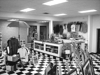 |
 |
 |
 |
 InsideCity |
 Kitchen |
 LivingRoom |
 Bedroom |
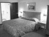
| Bedroom | 0.420 | 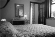 |
 |
 |
 |
 Highway |
 Kitchen |
 Kitchen |
 Store |
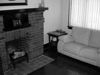
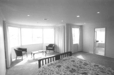
| LivingRoom | 0.270 | 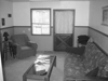 |
 |
 |
 |
 OpenCountry |
 InsideCity |
 Bedroom |
 Store |
| Office | 0.820 |  |
 |
 |
 |
 Kitchen |
 LivingRoom |
 LivingRoom |
 Kitchen |
| Industrial | 0.530 | 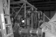 |
 |
 |
 |
 InsideCity |
 Street |
 Coast |
 Highway |
| Suburb | 0.930 |  |
 |
 |
 |
 OpenCountry |
 OpenCountry |
 InsideCity |
 Highway |
| InsideCity | 0.430 |  |
 |
 |
 |
 Highway |
 TallBuilding |
 Industrial |
 Industrial |
| TallBuilding | 0.640 |  |
 |
 |
 |
Industrial |
Industrial |
 Industrial |
 Store |
| Street | 0.640 |  |
 |
 |
 |
 Bedroom |
 TallBuilding |
 LivingRoom |
 InsideCity |
| Highway | 0.790 |  |
 |
 |
 |
 OpenCountry |
 OpenCountry |
 OpenCountry |
 InsideCity |
| OpenCountry | 0.460 |  |
 |
 |
 |
 Coast |
 Mountain |
 Suburb |
 Coast |
| Coast | 0.820 |  |
 |
 |
 |
 OpenCountry |
 Industrial |
OpenCountry |
 OpenCountry |
| Mountain | 0.790 |  |
 |
 |
 |
 Forest |
 Forest |
 Highway |
 Forest |
| Forest | 0.960 |  |
 |
 |
 |
 OpenCountry |
 OpenCountry |
 Mountain |
| Category name | Accuracy | Sample training images | Sample true positives | False positives with true label | False negatives with wrong predicted label | ||||
Extra Points Implementation
1. Soft Assignment for creating histogram
Instead of using the nearest neighbor for classfying features into clusters, each feature casts a vote on each cluster as long as it is near enough to the cluster center. In practice, the feature gives a vote with value 1 to its nearest cluster center. It will also give a vote with the value to every other cluster based on the ratio of the distance between feature and nearest cluster center and the distance between feature and the corresponding cluster center. This ratio is thresholded at the level of 0.8 to prevent giving out too many votes to completely irrevelant clusters. The accuracy is boosted by a bit, reaching 67% eventually.
Scene classification results visualization
Accuracy (mean of diagonal of confusion matrix) is 0.667
| Category name | Accuracy | Sample training images | Sample true positives | False positives with true label | False negatives with wrong predicted label | ||||
|---|---|---|---|---|---|---|---|---|---|
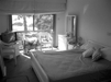
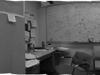
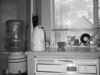
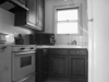
| Kitchen | 0.500 |  |
 |
 |
 |
 Industrial |
 Bedroom |
 Bedroom |
 Industrial |
| Store | 0.540 |  |
 |
 |
 |
 Kitchen |
 LivingRoom |
 Bedroom |
 Kitchen |
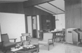
| Bedroom | 0.490 |  |
 |
 |
 |
 Office |
Kitchen |
 Kitchen |
 LivingRoom |
| LivingRoom | 0.320 |  |
 |
 |
 |
 Industrial |
 Bedroom |
 Street |
 Bedroom |
| Office | 0.770 |  |
 |
 |
 |
 Bedroom |
 Store |
 Bedroom |
 Kitchen |
| Industrial | 0.550 |  |
 |
 |
 |
 Street |
 Kitchen |
 Highway |
 Suburb |
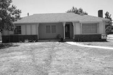
| Suburb | 0.950 | 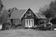 |
 |
 |
 |
 LivingRoom |
 Bedroom |
 Industrial |
 Coast |
| InsideCity | 0.580 |  |
 |
 |
 |
 Store |
 Street |
 Mountain |
 Kitchen |
| TallBuilding | 0.700 |  |
 |
 |
 |
 Store |
 Street |
 Street |
 Kitchen |
| Street | 0.650 |  |
 |
 |
 |
 Highway |
TallBuilding |
 Highway |
 Industrial |
| Highway | 0.850 |  |
 |
 |
 |
 Coast |
 Coast |
 TallBuilding |
 InsideCity |
| OpenCountry | 0.600 |  |
 |
 |
 |
 Industrial |
 Industrial |
 TallBuilding |
 Mountain |
| Coast | 0.740 |  |
 |
 |
 |
 Highway |
 OpenCountry |
 OpenCountry |
 Mountain |
| Mountain | 0.810 |  |
 |
 |
 |
 OpenCountry |
 Industrial |
 Suburb |
 Suburb |
| Forest | 0.950 |  |
 |
 |
 |
 Mountain |
 Mountain |
 Industrial |
 Mountain |
| Category name | Accuracy | Sample training images | Sample true positives | False positives with true label | False negatives with wrong predicted label | ||||
2. Cross Validation
I have used cross validation for reporting the performance of the system. 100 training and testing images are randomly picked in each iteration. Average accuracy and standard deviation are reported. However, cross-validation runs pretty slow as it requires a few iterations of training. I have only run the algorithm for reporting accuracy for tiny images with nearest neighbor, and bags of SIFT features with svm. The result is visualized in the following table.
| # | Tiny Images with Nearest Neighbor | Bags of SIFT with Support Vector Machine |
|---|---|---|
| 1 | 0.231 | 0.672 |
| 2 | 0.243 | 0.683 |
| 3 | 0.223 | 0.685 |
| 4 | 0.215 | 0.677 |
| 5 | 0.223 | 0.669 |
| 6 | 0.216 | 0.676 |
| 7 | 0.224 | 0.670 |
| 8 | 0.231 | 0.677 |
| 9 | 0.241 | 0.661 |
| 10 | 0.235 | 0.681 |
| Mean | 0.2282 | 0.6751 |
| Standard Deviation | 0.0097 | 0.0073 |
The system presents pretty stable performance upon the cross validation.
3. Performance for different vocabulary size
I have done some experiments with the vocabulary size used and evaluated the accuracy. The experiment is on the bags of SIFT features with soft assignment and svm classifier. The result is shown in the following table.
| Vocabulary Size | Accuracy | Average time for obtaining feature histogram for 100 images (s) |
|---|---|---|
| 10 | 0.405 | 9.634 |
| 20 | 0.536 | 9.344 |
| 50 | 0.595 | 10.672 |
| 100 | 0.642 | 12.602 |
| 200 | 0.650 | 17.846 |
| 500 | 0.669 | 31.363 |
| 1000 | 0.671 | 50.303 |
| 10000 | 0.653 | 337.792 |
As the table shows, the accuracy increases as the vocabulary size increases, but capped at around 65% to 70%. When the vocabulary size reaches 100, the accuracy hardly increase as the vocabulary size increases. Therefore, the best accuracy that this system can probably achieve is around 65% to 70%. The running time increases a lot as the vocabulary increases. Given that the accuracy performance does not change a lot, it is probably unwise to keep a huge vocabulary.
4. Performance on multiple scales
I have also done some experiments with the scale of the image. The image gets gaussian blurred in each scale and the corresponding accuracy is reported in the following table.
| Sigma | Accuracy |
|---|---|
| 0 (Unblurred) | 0.671 |
| 2^0.5 | 0.577 |
| 2^1.0 | 0.553 |
| 2^1.5 | 0.509 |
| 2^2.0 | 0.479 |
| 2^2.5 | 0.449 |
As the table shows, the accuracy of the recoginition drops by a few percent in each level. As the images are gradually losing high-ferequency information, it makes sense that the accuracy is in a decreasing trend.