Recognition with Bag of Words

Project 4 / Scene Recognition with Bag of Words

This project invovled classifying a grayscale image based on its scene. At first features were generated using images themselves reseized to a small size, and were then classified using KNN. More accurate classifications were made by utilizing a bag of SIFT feature, and also by using an SVM to classify the images.

Tiny Images and 1-NN

The tiny image feature was created by resizing all the images to be 16x16. Test images were classified by first resizing it to 16x16, and then finding its nearest neighbor in the training set. The category of the nearest neighbor was assigned to that test instance.

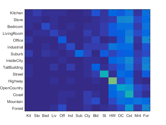
This resulted in a test accuracy of 0.201, which is greater than the chance of randomly selecting a correct label, which is 0.07.

Bag of SIFT and KNN

The bag of SIFT feature was created by first creating a visual vocabulary by using K-Means to find clusters of SIFT features in the training set. Bags of SIFT were created by finding the nearest vocabulary match for each SIFT feature, and then creating a histogram representing the amount of each vocabularly entry seen in every image. These features were then used with KNN to determine a category for every test image. A sift step-size of 40 was first tested.

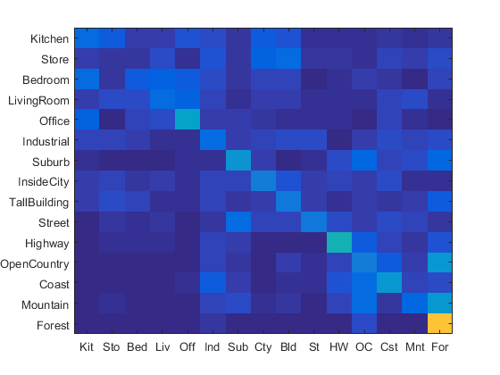
This resulted in an accuracy of .263, due to the low resolution used in sampling for SIFT features.

Decreasing the step size to 10 and therefore increasing resolution, the accuracy is much higher at 0.495.

Bag of SIFT and SVM

This time, instead of using a nearest neighbor classfier, an SVM was used to classify the test images. One SVM was trained per each of the 15 categories, using the bag of SIFT features as an input. When determining a category for a test image, the category of the SVM which output the highest score was taken to be the test image's category.

In order to tune the SVM hyperparameters, a bag of SIFT feature with SIFT features found with a step size of 40 was used as an input to tune the epsilon parameter of the SVMs. The results are as follows:

lambda	Accuracy
0.00001	0.329
0.0001	0.380
0.001	0.403
0.01	0.375
0.01	0.375
0.1	0.386
1	0.375

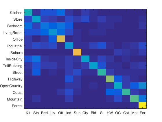
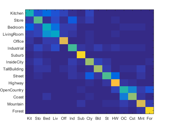
As seen, a lambda value of 0.001 provides the best results, and was therefore used for the rest of the runs. Decreasing the SIFT step size to 20, the accuracy was increased to 0.533. Further reducing to 10 led to a 0.633 accuracy, with the heatmap shown below.

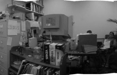
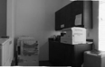
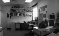
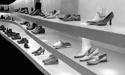
Category name	Accuracy	Sample training images	Sample true positives	False positives with true label		False negatives with wrong predicted label
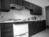
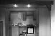
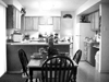
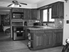
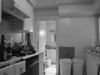
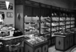
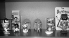
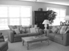
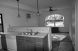
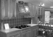
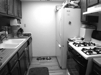
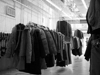
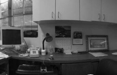
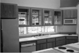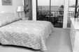
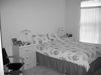
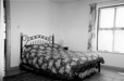
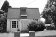
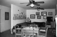
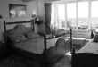
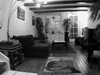
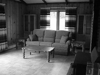
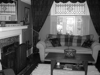
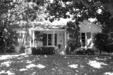
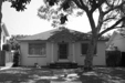
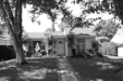
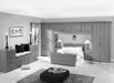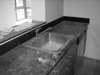
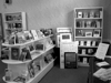
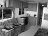
Kitchen	0.530			Bedroom	Store	InsideCity	Office
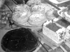
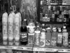
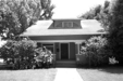
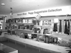
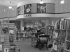
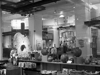
Store	0.420		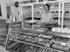	InsideCity	InsideCity	Industrial	InsideCity
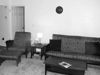
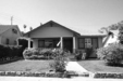
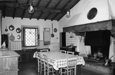
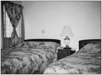
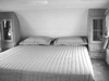
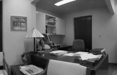
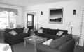
Bedroom	0.340			Kitchen	LivingRoom	TallBuilding	Mountain
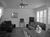
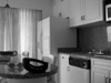
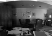
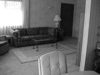
LivingRoom	0.250			Industrial	Bedroom	Bedroom	Kitchen
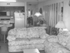
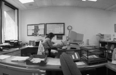
Office	0.940		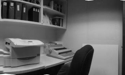	Mountain	LivingRoom	Kitchen	Bedroom
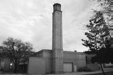
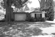
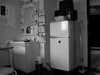
Industrial	0.360			Store	InsideCity	Suburb	TallBuilding
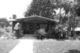
Suburb	0.950		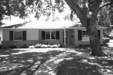	Coast	Forest	Coast	TallBuilding
InsideCity	0.600			Kitchen	TallBuilding	TallBuilding	Industrial
TallBuilding	0.770			Industrial	Street	InsideCity	Highway
Street	0.620			Bedroom	Bedroom	Highway	Mountain
Highway	0.780			Coast	Store	Office	Coast
OpenCountry	0.330			Coast	Street	Forest	Highway
Coast	0.840			OpenCountry	OpenCountry	Mountain	Mountain
Mountain	0.840			Industrial	Coast	Forest	Forest
Forest	0.930			OpenCountry	OpenCountry	Street	Mountain
Category name	Accuracy	Sample training images	Sample true positives	False positives with true label		False negatives with wrong predicted label

Further Improving Accuracy

Different Vocabulary Size

To investigate the effects of changing the vocabulary size, different sizes were used when generating the bag of SIFT features that were used in the SVM classifier. As seen below, increasing the vocabulary size only increases the accuracy up to a certain extent, and then goes on to reduce the accuracy as the size is increased. This may be due to the fact that as more clusters are used when finding the vocabulary, more noise is captured from the training SIFT features.

Vocab Size	Accuracy
10	0.315
20	0.333
50	0.371
100	0.404
200	0.407
400	0.406
1000	0.403

Fisher Encoding

Fisher encoding was done by first creating a Gaussian mixture model from all the SIFT features found in the training set.


%example code
stepsize = 10;
for k = 1:length(image_paths)
    im = imread(image_paths{k});
    [locations, SIFT_features] = vl_dsift(single(im), 'step', stepsize, 'fast');
    sift_features = [sift_features SIFT_features];
end
sift_features = single(sift_features);
numClusters = 30;
[means, covariances, priors] = vl_gmm(single(sift_features), numClusters);

Then the fisher encoding for the SIFT features found in each image was calculated using this GMM.


 stepsize = 10
 image_feats = [];

 for k = 1:length(image_paths)
 	im = imread(image_paths{k});
	[locations, SIFT_features] = vl_dsift(single(im), 'step', stepsize, 'fast' );

 	sift_feats = vl_fisher(single(SIFT_features), means, covariances, priors)';
 end

The Fisher encoded vector was used in place of the histogram generated from the vocabulary file when training the SVMs. Using the Fisher encoded vector instead of the bag of SIFT feature with an SVM with lambda value of 0.001 resulted in an accuracy of 0.631, a slight decrease compared to the bag of SIFT + SVM accuracy value of 0.633.

GIST Features

The addition of GIST features was also tested. These GIST features were used in addition to the bag of SIFT feature as an input when training the SVMs.


    %Get GIST descriptors
    clear param
    param.orientationsPerScale = [8 8 8 8]; % number of orientations per scale (from HF to LF)
    param.numberBlocks = 4;
    param.fc_prefilt = 4;
    [gist, param] = LMgist(im, '', param);

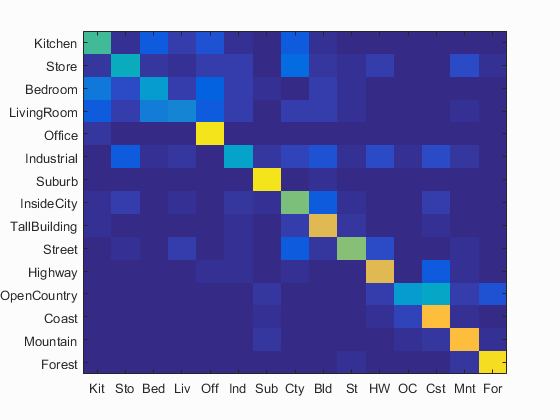
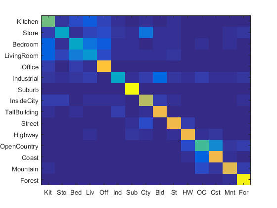
Combining GIST with Fisher vector features resulted in an accuracy of 0.669, an improvement over only using Fisher vectors as features. Combining GIST features with bag of SIFT features provided a much more noticible improvement in accuracy, with the accuracy jumping to 0.740. The heatmap for GIST + bag of SIFT was shown below. The GIST parameters are shown above, the SIFT step size was 10, and the SVM lambda was 0.001.

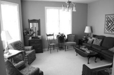
Category name	Accuracy	Sample training images	Sample true positives	False positives with true label		False negatives with wrong predicted label
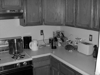
Kitchen	0.590		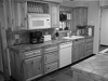	InsideCity	LivingRoom	LivingRoom	Bedroom
Store	0.380			Kitchen	InsideCity	Street	InsideCity
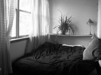
Bedroom	0.390			Kitchen	LivingRoom	Kitchen	Industrial
LivingRoom	0.320		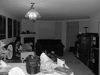	Store	Kitchen	Store	Street
Office	0.850		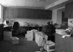	Store	Kitchen	Suburb	Kitchen
Industrial	0.390			InsideCity	Store	InsideCity	TallBuilding
Suburb	0.990		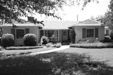	Store	Highway	LivingRoom
InsideCity	0.690			Store	Store	Highway	TallBuilding
TallBuilding	0.800			Industrial	Industrial	Store	Kitchen
Street	0.810			Store	Highway	Industrial	InsideCity
Highway	0.810			OpenCountry	Street	Industrial	Street
OpenCountry	0.520			Coast	Mountain	Forest	Coast
Coast	0.800			OpenCountry	OpenCountry	Highway	Highway
Mountain	0.770			Store	Kitchen	LivingRoom	Kitchen
Forest	0.970			OpenCountry	Store	Mountain	Mountain
Category name	Accuracy	Sample training images	Sample true positives	False positives with true label		False negatives with wrong predicted label

Henry Chen