Project 4 / Scene Recognition with Bag of Words

In this project, I implemented the following:

1. Tiny Image + k-NN
2. Bag of SIFT + k-NN
3. Bag of SIFT + SVM
4. (Extra Credit) Bag of SIFT + non-linear SVM with RBF kernel
5. (Extra Credit) Bag of SIFT + Gist Descriptor + SVM

Apart from all the above, I tested all the algorithms using cross validation. The details of parameter selection will be discussed there.

Finally, I've included a brief summary of observations at the very end.

Tiny Image + k-NN

In this part, I resized the image to 16x16 tiny ones, which are used as features. The k-NN classifier uses L2-distance. By trail and error, I set k = 9, which gives accuracy of 21.4%.

Result: Tiny Image + k-NN

Scene classification results visualization

Accuracy (mean of diagonal of confusion matrix) is 0.214

Category name	Accuracy	Sample training images		Sample true positives		False positives with true label		False negatives with wrong predicted label
Kitchen	0.050					Office	Office	Bedroom	Bedroom
Store	0.010					Bedroom	Kitchen	OpenCountry	LivingRoom
Bedroom	0.160					Kitchen	LivingRoom	Kitchen	Coast
LivingRoom	0.060					Forest	Industrial	Highway	Bedroom
Office	0.120					Suburb	InsideCity	LivingRoom	Street
Industrial	0.070					Office	Kitchen	Coast	Highway
Suburb	0.370					Kitchen	Coast	OpenCountry	Highway
InsideCity	0.070					OpenCountry	Coast	Coast	Office
TallBuilding	0.120					Store	Office	Bedroom	Highway
Street	0.490					Store	Store	Industrial	Coast
Highway	0.730					OpenCountry	TallBuilding	OpenCountry	Coast
OpenCountry	0.300					InsideCity	Mountain	Suburb	Coast
Coast	0.340					InsideCity	Store	Mountain	Highway
Mountain	0.190					Coast	Bedroom	Coast	Coast
Forest	0.130					Store	Highway	Highway	Coast
Category name	Accuracy	Sample training images		Sample true positives		False positives with true label		False negatives with wrong predicted label

Bag of SIFT + k-NN

In this part, I collected the SIFT features from both train and test images. Using the SIFT features from train images, I ran k-means to obtain a vocabulary of "visual words". With this vocabulary, the SIFT features of each image (in both train and test sets) are classfied into the closet "visual word" in L2-metric, and then the histogram of number of words in each image is generated as bag of SIFT feature.

If every SIFT feature is retained for each image, then there will be around 50k SIFT feature vectors per image. The runtime of k-means on the training set (1500 images) will take long time. Thus, I used 'fast' argument in vl_dsift function. Also, I adjusted the sampling density of SIFT features by setting the minimum distance between each SIFT feature to 8 pixels, using the code below. The sampling density for test set was not changed to ensure accuracy.

	
	[loc, feat] = vl_dsift(single(imread(image_paths{i+prev_count})), 'fast', 'step', 8);
	

For the k-means, number of clusters is set to 200 (as in the default code). k was set to 9 as before.

With only around 1/8 of the training data (because of the lowered sampling density), the algorithm still gives good accuracy of 55.1%.

Result: Bag of SIFT + k-NN

Scene classification results visualization

Accuracy (mean of diagonal of confusion matrix) is 0.551

Category name	Accuracy	Sample training images		Sample true positives		False positives with true label		False negatives with wrong predicted label
Kitchen	0.460					Office	Store	LivingRoom	LivingRoom
Store	0.500					InsideCity	InsideCity	Bedroom	LivingRoom
Bedroom	0.400					LivingRoom	LivingRoom	Store	Store
LivingRoom	0.530					TallBuilding	Bedroom	Bedroom	Store
Office	0.730					LivingRoom	Bedroom	LivingRoom	LivingRoom
Industrial	0.340					InsideCity	LivingRoom	Store	Kitchen
Suburb	0.850					OpenCountry	Mountain	Store	InsideCity
InsideCity	0.460					Bedroom	Kitchen	Store	Store
TallBuilding	0.250					Bedroom	Bedroom	Store	Street
Street	0.650					TallBuilding	TallBuilding	Store	InsideCity
Highway	0.820					Coast	OpenCountry	Coast	InsideCity
OpenCountry	0.390					Industrial	Coast	Mountain	Forest
Coast	0.460					OpenCountry	TallBuilding	Highway	Suburb
Mountain	0.470					OpenCountry	Highway	Bedroom	Highway
Forest	0.950					Mountain	Mountain	Mountain	Suburb
Category name	Accuracy	Sample training images		Sample true positives		False positives with true label		False negatives with wrong predicted label

Bag of SIFT + SVM

In this part, I used SVM to classify bag of SIFT features, instead of k-NN. Using 1-vs-all approach, the each category a SVM was trained to tell if one image is of this category or not. The final prediction is generated by taking the category with maximum score. The bag of SIFT features are generated as before.

By trail and error, I set lambda (the regularization constant) to 5. Also, to ensure numerical stability, I set the number of iterations to be 10000. This algorithm gives 68% accuracy.

Scene classification results visualization

Accuracy (mean of diagonal of confusion matrix) is 0.680

Category name	Accuracy	Sample training images		Sample true positives		False positives with true label		False negatives with wrong predicted label
Kitchen	0.550					Store	InsideCity	LivingRoom	Office
Store	0.560					InsideCity	Bedroom	InsideCity	Bedroom
Bedroom	0.450					LivingRoom	LivingRoom	Kitchen	Kitchen
LivingRoom	0.390					Kitchen	Bedroom	Bedroom	TallBuilding
Office	0.900					Kitchen	Bedroom	Kitchen	Street
Industrial	0.570					LivingRoom	Bedroom	LivingRoom	Mountain
Suburb	0.950					Highway	OpenCountry	Street	Industrial
InsideCity	0.500					TallBuilding	Store	Bedroom	TallBuilding
TallBuilding	0.830					Industrial	Street	Industrial	Coast
Street	0.610					Bedroom	Industrial	Store	Industrial
Highway	0.820					Coast	OpenCountry	OpenCountry	Coast
OpenCountry	0.550					Coast	Coast	Street	Coast
Coast	0.780					OpenCountry	Highway	Highway	Highway
Mountain	0.800					Forest	Store	OpenCountry	OpenCountry
Forest	0.940					Mountain	Highway	InsideCity	Street
Category name	Accuracy	Sample training images		Sample true positives		False positives with true label		False negatives with wrong predicted label

Bag of SIFT + non-linear SVM with RBF kernel

In this part, I trained the features using non-linear SVM with RBF kernel, for which I used sklearn.svm.SVC class in scikit-learn library. Since RBF kernel has much more degree of freedom, the regularization value for SVM should be set to larger value to prevent overfitting on the relatively small dataset. Also, the gamma value determines the spread of the kernel function (inversely proportional to sigma^2). The performance is sensative to this value. By trail and error, I set lambda = 1000 and gamma = 2. This algorithm gives accuracy of 70.7%.

Scene classification results visualization

Accuracy (mean of diagonal of confusion matrix) is 0.707

Category name	Accuracy	Sample training images		Sample true positives		False positives with true label		False negatives with wrong predicted label
Kitchen	0.650					Store	Office	InsideCity	Office
Store	0.620					LivingRoom	Suburb	LivingRoom	Bedroom
Bedroom	0.630					InsideCity	Kitchen	LivingRoom	LivingRoom
LivingRoom	0.450					Bedroom	Kitchen	Store	Office
Office	0.850					Kitchen	Bedroom	LivingRoom	Kitchen
Industrial	0.610					LivingRoom	Street	Street	Coast
Suburb	0.900					Street	Mountain	Industrial	Highway
InsideCity	0.630					Street	Store	Store	Industrial
TallBuilding	0.750					Industrial	Industrial	Kitchen	Store
Street	0.710					Industrial	InsideCity	TallBuilding	Suburb
Highway	0.810					OpenCountry	LivingRoom	Coast	OpenCountry
OpenCountry	0.580					Coast	Coast	Forest	Coast
Coast	0.760					OpenCountry	OpenCountry	OpenCountry	OpenCountry
Mountain	0.750					Forest	Kitchen	TallBuilding	OpenCountry
Forest	0.900					OpenCountry	Mountain	Mountain	Mountain
Category name	Accuracy	Sample training images		Sample true positives		False positives with true label		False negatives with wrong predicted label

Bag of SIFT + Gist Descriptors + SVM

In this part, I added Gist descriptors along with bag of SIFT features. Gist descriptors, different than SIFT, describe the global feature of one image.

To combine these two kinds of features, I simply appended Gist descriptors to the bag of SIFT features. However, these two heterogeous features have difference in scale. In my case (using 200 vocab size), the L2-norm of bag of SIFT features can be over 70 but that of Gist descriptor is lower than 1. Therefore, I scaled the Gist descriptors by some constant so that they can match. In my case, I set the constant to 500.

The settings of SVM were the same. This algorithm gives accuracy around 77% (it fluctuates a little bit due to the randomness in the SVM solver).

Scene classification results visualization

Accuracy (mean of diagonal of confusion matrix) is 0.768

Category name	Accuracy	Sample training images		Sample true positives		False positives with true label		False negatives with wrong predicted label
Kitchen	0.590					TallBuilding	Bedroom	Store	Store
Store	0.650					Industrial	Bedroom	Kitchen	Kitchen
Bedroom	0.660					Kitchen	LivingRoom	LivingRoom	Store
LivingRoom	0.590					Bedroom	Kitchen	Bedroom	Kitchen
Office	0.880					Store	Kitchen	Kitchen	Kitchen
Industrial	0.670					Store	Store	TallBuilding	LivingRoom
Suburb	0.950					Bedroom	OpenCountry	Industrial	Industrial
InsideCity	0.820					TallBuilding	Street	Industrial	Street
TallBuilding	0.780					InsideCity	InsideCity	Kitchen	Forest
Street	0.860					InsideCity	Highway	Mountain	InsideCity
Highway	0.860					Coast	OpenCountry	Suburb	Coast
OpenCountry	0.750					Coast	Industrial	Highway	Mountain
Coast	0.730					Mountain	OpenCountry	OpenCountry	Street
Mountain	0.810					Forest	TallBuilding	Highway	Coast
Forest	0.920					Mountain	OpenCountry	Mountain	OpenCountry
Category name	Accuracy	Sample training images		Sample true positives		False positives with true label		False negatives with wrong predicted label

Cross Validation

In this part, I separated the orginal dataset into two halfs. The first half is the validation dataset and the other half becomes the new test set. I ran the above algorithms on validation set to select the best parameters. Then I test this parameter setting on the clean test dataset. The best validation accuracy is in the title of each plot.

Bag of SIFT + k-NN

The result on picking best k:

Using the best set of parameters, test accuracy = 54.3%

Bag of SIFT + linear SVM

The result on picking best lambda:

Using the best set of parameters, test accuracy = 66.9%

Bag of SIFT + non-linear SVM

Since we have two parameters, I first fix gamma = 2 and pick the best lambda. Then I fixed lambda to be the best one (when gamma = 2) and pick the best lambda.

The result on picking best lambda:

The result on picking best gamma:

Using the best set of parameters, test accuracy = 69.9%

Bag of SIFT + Gist Descriptors + SVM

The result on picking best lambda:

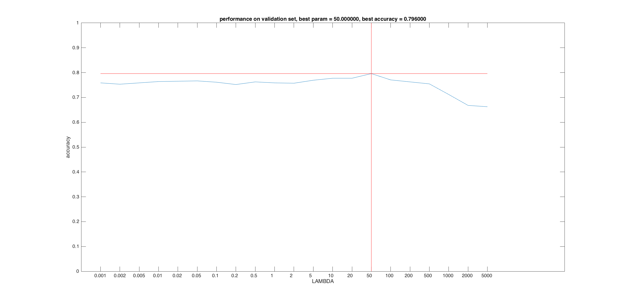
Using the best set of parameters, test accuracy = 76.0%

Observation