Project 4 / Scene Recognition with Bag of Words

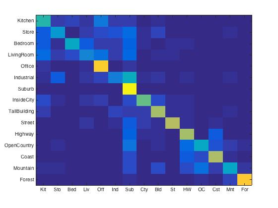
Confusion matrix for vocab_size = 400, using SVM classifier.
This project is to implement image recognition with different methods. First, we will use a simple method: tiny image (16x16) with nearest neighbor. Then we replace the image represenntation with bag of features. Finally, we use SVM instead of nearest neighbor as the classifier. So there are basically three steps:
- tiny images + nearest neighbor
- bag of features + nearest neighbor
- bag of features + SVM
In order to use bag of features to represent images, we need to build a vocabulary using the training images. This default size is set to 200. In extra credit part, I tested the size of 10, 50, 100, 200 and 400. The result will be shown in later section.
Algorithm
- Tiny images: resize each image to 16x16 size, normalize it to zero mean and unit length.
- Nearest neighbor: Simply calculate pairwise Euclidean distance, select the closest one as the image's prediction.
- Vocabulary construction: Use K-means to cluster the samples of SIFT from training images.
- Bag of SIFT: Sample SIFT discriptors, cluster them to the cloest centroid from the vocabulary. Calculate the histogram of discriptors in each bin and normalized it.
- SVM: Train a linear SVM for each category, then use it to predict each image. Select the category with the highest confidence.
Core Code
% tiny image
for i = 1 : num
  image_feat = single(imresize(imread(image_paths{i}), [dim, dim]));
  image_feat = bsxfun(@minus, image_feat, mean(image_feat));
  image_feat = image_feat ./ std2(image_feat);
  image_feats(i, :) = reshape(image_feat, [1, dim * dim]);
end

% nearest neighbor
Dist = vl_alldist2(train_image_feats', test_image_feats');
[~, I] = min(Dist);
...
for i = 1 : num
    predicted_categories{i} = train_labels{I(i)};
end

% vocabulary construction
for i = 1 : num
    data = single(imread(image_paths{i}));
    [~, features] = vl_dsift(data,'step', 5);
    sample = horzcat(sample, features);
end
[vocab, ~] = vl_kmeans(single(sample), vocab_size);

% bag of SIFT
for i = 1 : num
	[locations, features] = vl_dsift(A, 'step', 5);
	D = vl_alldist2(vocab, single(features));
	[~, I] = min(D);
	num_features = size(I, 2);
	for j = 1 : num_features
	    image_feats_0(i, I(j)) = image_feats_0(i, I(j)) + 1;
	end
end

% linear svm
for i = 1 : num_categories
    matching_indices = strcmp(categories{i}, train_labels);
    matching_indices = matching_indices * 2 - 1;
    [W(:, i), B(1, i)] = vl_svmtrain(train_image_feats, double(matching_indices), LAMBDA);
end

for i = 1 : num_images
   for j = 1 : num_categories
       score(1, j) = test_image_feats(i, :) * W(:, j) + B(1, j);
   end
   [~, index] = max(score);
   predicted_categories{i} = categories{index};
end
Extra credit
- Tested different vocabulary sizes: 10, 50, 100, 200, 400.
- Implemented spatial pyramid and pyramid match kernel.
Core Code
% spatial_pyramid.m
sp_size = 2 ^ level;
for row_part = 1 : sp_size
    for col_part = 1 : sp_size
        [~, features] = vl_dsift(image((row_part - 1) * floor(length / sp_size) + 1 : row_part * floor(length / sp_size),...
            (col_part - 1) * floor(width / sp_size) + 1 : col_part * floor(width / sp_size)),'step', 5);
        D = vl_alldist2(vocab, single(features));
        [~, I] = min(D);
        num_features = size(I, 2);
        for j = 1 : num_features
            %center
            temp_feats(I(j)) = temp_feats(I(j)) + 1;
        end
        image_feats(part * vocab_size + 1 : (part + 1) * vocab_size) = temp_feats(1 : vocab_size);
        temp_feats = zeros(1, vocab_size);
        part = part + 1;
    end
end
Results
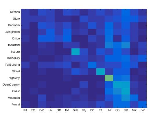
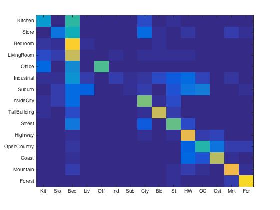
Tiny image + Nearest neighbor. Images were resized to 16x16, the accuracy was 20.3%, which is really bad. This is reasonable, because we lost a lot of high frequency information when we resize the images to small patches.
|
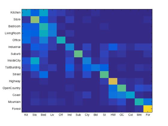
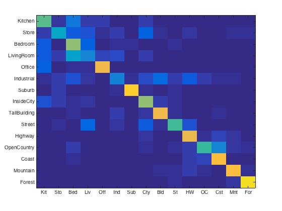
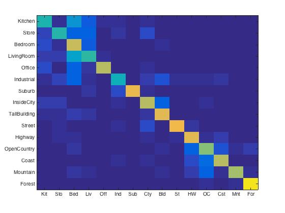
Bag of SIFT + Nearest neighbor. To speed up the process, I set step size to 5 in vl_dsift and the vocabulary size was 200. The accuracy was 46.3%. Compare to the tiny image representation method, we kept more information. Apparently, we represented the images better. However, the classifier is still too simple to reach a satisfying accuracy.
|
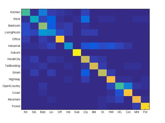
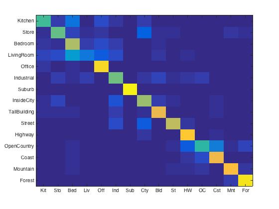
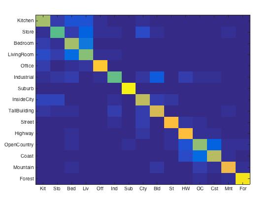
Bag of SIFT + Linear SVM. Here I set the step size to 5, vocabulary size to 200, and I found the best lambda is 0.00001. With these parameteres, I got the best accuracy, 67.4%. Though it seems better than the two method above, it could still be improved by larger vocabulary size or use spatial pyramid. I'll show that in next section for extra credit part.
|
Extra credit part
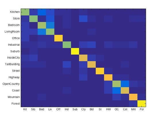
For different vocabluary size, I got following results. The accruacy were 23.6%, 50.7%, 64.1% 67.4%, 70.4% for size of 10, 50, 100, 200, 400, respectively. As you can see, the accuracy increased significantly from size of 10 to 50, and 50 to 100. Since the running time increases dramatically with the vocab_size, the largest size I tested was 400. And it gave acceptable accuracy as shown below.
|
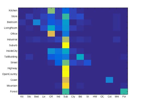
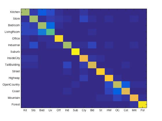
After I implemented 3 level spatial pyramid (1x1, 2x2, 4x4) and pyramid match kernel. I also tested it with different vocabulary sizes. The accruacy were 56.6%, 66.9%, 74.3% 76.6%, 77.8% for size of 10, 50, 100, 200, 400, respectively. Compare to the data above, one interesting thing is there is a big improvement for size of 10. And the best accuracy I got (at size of 400) also reached 77.8%, which is good for a linear SVM classifier.
|
Project 4 results visualization
This is the best result I could get. I implemented it with 3 level spatial pyramid and vocabulary size 400.

Accuracy (mean of diagonal of confusion matrix) is 76.6%
| Category name | Accuracy | Sample training images | Sample true positives | False positives with true label | False negatives with wrong predicted label | ||||
|---|---|---|---|---|---|---|---|---|---|
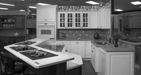
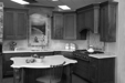
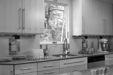
| Kitchen | 0.640 | 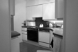 |
 |
 |
 |
 OpenCountry |
 InsideCity |
 Bedroom |
 LivingRoom |
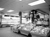
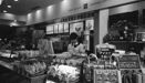
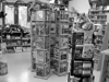
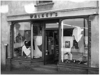
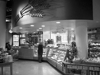
| Store | 0.610 |  |
 |
 |
 |
 TallBuilding |
 Industrial |
 InsideCity |
 Forest |
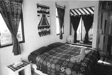
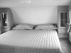
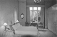
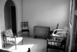
| Bedroom | 0.660 | 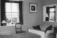 |
 |
 |
 |
 Store |
 LivingRoom |
 Kitchen |
 Industrial |
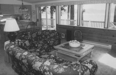
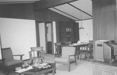
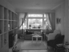
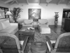
| LivingRoom | 0.630 | 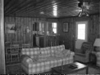 |
 |
 |
 |
 Store |
 Store |
 Bedroom |
 Bedroom |
| Office | 0.890 |  |
 |
.jpg) |
 |
 LivingRoom |
 InsideCity |
 LivingRoom |
 LivingRoom |
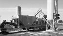
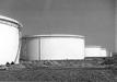
| Industrial | 0.620 | 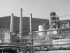 |
 |
 |
 |
 TallBuilding |
 Store |
 OpenCountry |
 Highway |
| Suburb | 0.970 |  |
 |
 |
 |
 Store |
 Industrial |
 Store |
 Store |
| InsideCity | 0.780 |  |
 |
 |
 |
 Highway |
 Highway |
 TallBuilding |
Kitchen |
| TallBuilding | 0.780 |  |
 |
 |
 |
 Store |
 Store |
 Industrial |
 Forest |
| Street | 0.880 |  |
 |
 |
 |
 InsideCity |
 LivingRoom |
 Store |
 Highway |
| Highway | 0.840 |  |
 |
 |
 |
Street |
 Store |
 Store |
InsideCity |
| OpenCountry | 0.660 |  |
 |
 |
 |
 Highway |
 Coast |
 Forest |
 Mountain |
| Coast | 0.750 |  |
 |
 |
 |
 OpenCountry |
 OpenCountry |
 Highway |
 OpenCountry |
| Mountain | 0.820 | .jpg) |
 |
 |
 |
 Kitchen |
 Store |
 OpenCountry |
 OpenCountry |
| Forest | 0.960 |  |
 |
 |
 |
 OpenCountry |
 Mountain |
 Mountain |
 Mountain |
| Category name | Accuracy | Sample training images | Sample true positives | False positives with true label | False negatives with wrong predicted label | ||||