Project 4 / Scene Recognition with Bag of Words
In this project, we build a scene recognition tool using the bag of words model. A scene recognizer learns from example images and classifies unseen images into the different scene classes learned. We start by using simple strategies such as the tiny images representation, and incrementally improve the algorithm by adding more sophisticated techniques.
This write-up will present the results in the order which they have been developed. Improvements in accuracy made along these iterations will also be discussed. All results shown uses the 'fast' argument in vlfeat's dense SIFT computation.
Baseline Results
The baseline of this project consists of the following stages:
- Tiny images representation and nearest neighbor classifier
- Bags of quantized SIFT features and nearest neighbor classifier
- Bags of quantized SIFT features and linear SVM classifier
To start off this project, the tiny images representation was used where we simply resize the image into a 16 by 16 patch. For simplicity, we ignore the images' aspect ratios in this process. To classify unseen images, we feed the image representation into a 1-nearest neighbor classifier, where we classify an image by the class of the single closest image in our training set. This set-up achieved an accuracy of 22.5%. It is not amazing but does improve drastically from the 7% baseline.
Next we tried using the Bag of SIFT representation instead of tiny images. To achieve this, we first build a vocabulary of SIFT features by sampling our training images. To ensure a representative sample, we sample a virtually uniform number of samples from each image. The samples are then clustered using k-means, where k is our vocabulary size. Finally, we build the vocabulary using the cluster centers. In this section, we use vocabularies made from 50,000 SIFT samples.
Once we have the vocabulary set, we can quantize each image into a word histogram. We first sample a number of sift features for each image. Our dense SIFT computation uses a step size of 8, as suggested by Lazebnik et al. 2006. This gives us a couple hundred SIFT features for each image. Then we match each sift feature to the closest vocabulary image and increment the respective bin in the word histogram. Finally, we normalize the histogram and perform classification. Initially, using a vocabulary of 200 visual words and a step size of 10, our classifier achieved an accuracy of 51.0%.
The nearest neighbor classifier works fine for this problem but it can be prone to overfitting as it is very sensitive to outliers. To address this issue, we can use Support Vector Machines (SVM) instead, which is less sensitive to outliers. We use the same word histograms from the previous part, but train a one-vs-all SVM classifier for every class. The image will be classified as the class in which the respective classifier returns the highest confidence score, even if it is on the wrong side of the decision boundary. Using a lambda value of 0.0001 and the same parameters as above, we achieved an accuracy of 62.8%.
The table below summarizes the accuracies achieved in the baseline setups, using the parameters mentioned above. With some parameter tuning (step_size = 8, number of features sample to build vocabulary = 500,000, lambda = 0.0001), our 200-word SVM classifier achieves an accuracy of 65.0%.
| Set-up | Accuracy |
| Tiny Images + 1NN | 22.5% |
| SIFT Bag + 1NN | 51.0% |
| SIFT Bag + SVM | 62.8% |
Extra Credit Results
This section continues from the 65.0% accuracy we achieved earlier and incrementally builds up the accuracy by making decisive changes to our pipeline. We build the vocabulary using 500,000 SIFT samples and extract dense SIFT features with a step size of 8.
The size of the vocabulary set built can greatly affect the prediction accuracy. We experimented with different vocabulary sizes as shown below. The results verified that the accuracy increases as we increase the vocabulary size, but only up to a certain point. Also, we found that larger vocabulary sizes take much longer to compute.
| Vocabulary Size | 10 | 20 | 50 | 100 | 200 | 400 | 1000 | 10000 |
| Accuracy | 38.8% | 50.5% | 60.1% | 63.1% | 65.0% | 66.2% | 70.1% | 68.1% |
The above experiment suggests that 1000 vocabulary words gives the best result. However, due to issues with computation time, we will use a vocabulary of size 200 until the very end of this discussion.
The quantization step in the pipeline can be lossy and to ameliorate this problem, we can use soft assignment when assigning SIFT features to visual histograms. The kernel codebook encoding method casts a distance-weighted vote into multiple histogram bins, by exp(-gamma/2 * ||x-mu||^2). We first experimented the number of nearest neighbors considered and found 3 works best. We then tried different gamma values with 3 votes and found gamma=0.1 to be the best option.| Number of Nearest Neighbors | 1 (Baseline) | 2 | 3 | 4 | 5 | 10 |
| Accuracy | 65.0% | 67.4% | 67.7% | 67.3% | 66.1% | 64.3% |
| Gamma | Accuracy |
| 1.0 | 67.7% |
| 0.5 | 67.8% |
| 0.1 | 68.1% |
| 0.01 | 67.5% |
Up to this point, our pipeline completely disregards any kinds of spatial information. Although the bags of words model aims to reduce the variance caused by spatial details, completely ignoring spatial information may not be desirable. Lazebnik et al. 2006 introduces a spatial scheme where we partition the image into equally sized sub-regions, and quantize a histogram in each region. This is the "Single Level" approach and they have also introduced a "Spatial Pyramid" scheme where multiple single level vectors are combined together. We measured performance on both quantization schemes using a linear SVM classifier.
| L | Single Level | Pyramid |
| 0 (1x1) | 68.1% | 68.1% |
| 1 (2x2) | 69.5% | 70.3% |
| 2 (4x4) | 72.5% | 73.7% |
| 3 (8x8) | 71.9% | 73.5% |
We have reached the same conclusion as the original authors that a level-2 scheme gives us the best results. We will build on the level-2 pyramid scheme.
Lastly, we tried to modify our SVM classifier to use non-linear kernels because linear models may not be complex enough to fit our underlying model. In particular, we tried the gaussian kernel and various polynomial kernels.
| Kernel | Accuracy |
| Linear | 73.7% |
| Gaussian/RBF | 75.0% |
| Polynomial d=2 | 75.0% |
| Polynomial d=3 | 76.3% |
| Polynomial d=4 | 77.2% |
| Polynomial d=5 | 76.4% |
| Polynomial d=6 | 75.9% |
Surprisingly, the polynomial kernel performs much better than the Gaussian kernel for this problem. We found that the 4-th degree polynomial kernel works best.
Below, we show the full accuracy results for the pipeline above using a 1000-word vocabulary. This set-up achieves an accuracy of 78.0%
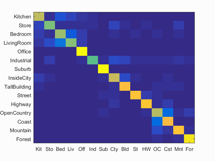
Accuracy (mean of diagonal of confusion matrix) is 0.780
| Category name | Accuracy | Sample training images | Sample true positives | False positives with true label | False negatives with wrong predicted label | ||||
|---|---|---|---|---|---|---|---|---|---|
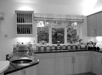
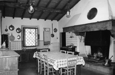
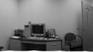
| Kitchen | 0.710 |  |
 |
 |
 |
 LivingRoom |
 TallBuilding |
 LivingRoom |
 Bedroom |
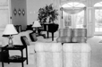
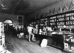
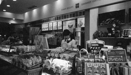
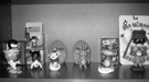
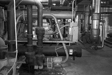
| Store | 0.600 | 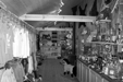 |
 |
 |
 Bedroom |
 Industrial |
 Office |
 Industrial |
|
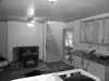
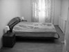
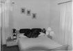
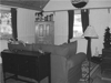
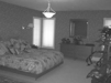
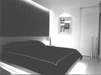
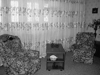
| Bedroom | 0.650 |  |
 |
 |
 |
 LivingRoom |
 LivingRoom |
 LivingRoom |
 Kitchen |
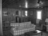
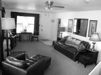
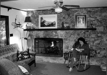
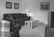
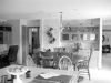
| LivingRoom | 0.610 |  |
 |
 |
 |
 Kitchen |
 Bedroom |
 Store |
Bedroom |
| Office | 0.990 | 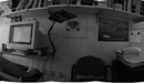 |
 |
 |
 |
 Bedroom |
 LivingRoom |
 Kitchen |
|
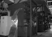
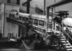
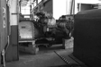
| Industrial | 0.550 | 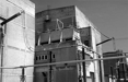 |
 |
 |
 |
 Store |
 Kitchen |
 Store |
 Mountain |
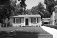
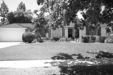
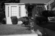
| Suburb | 0.990 | 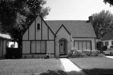 |
 |
 |
 |
 Industrial |
 Street |
 LivingRoom |
|
| InsideCity | 0.730 |  |
 |
 |
 |
 Highway |
 Store |
 Store |
 Kitchen |
| TallBuilding | 0.840 |  |
 |
 |
 |
 InsideCity |
 Industrial |
Kitchen |
 Kitchen |
| Street | 0.850 |  |
 |
 |
 |
 Industrial |
 LivingRoom |
 Highway |
 InsideCity |
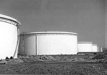
| Highway | 0.870 |  |
 |
 |
 |
 Industrial |
 Industrial |
 Coast |
 Coast |
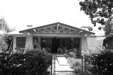
| OpenCountry | 0.700 |  |
 |
 |
 |
 Coast |
 TallBuilding |
 Forest |
 Mountain |
| Coast | 0.820 |  |
 |
 |
 |
 OpenCountry |
Highway |
 OpenCountry |
 OpenCountry |
| Mountain | 0.850 |  |
 |
 |
 |
 Forest |
 Store |
 Coast |
 Coast |
| Forest | 0.940 |  |
 |
 |
 |
 Store |
OpenCountry |
 OpenCountry |
 Suburb |
| Category name | Accuracy | Sample training images | Sample true positives | False positives with true label | False negatives with wrong predicted label | ||||
Finally, we verify the accuracy of our classifier using k-fold cross validation to ensure that we are not overfitting this particular test case. We performed 10-fold cross validation on the 200-word classifier:
| Fold | 1 | 2 | 3 | 4 | 5 | 6 | 7 | 8 | 9 | 10 |
| Accuracy | 77.93% | 77.80% | 77.87% | 78.20% | 77.00% | 79.53% | 77.13% | 78.47% | 78.87% | 78.53% |
| Mean Accuracy | 78.13% |
| Standard Deviation of Accuracy | 0.7659% |
The cross-validated accuracy happens to be better than the 77.2% in the baseline test case!!
List of extra credits mentioned in this report
- Kernel book encoding
- Train SVM with more sophisticated kernels
- Spatial pyramid feature representation
- Cross validation
- Experiment with different vocabulary sizes