Project 5 / Face Detection with a Sliding Window
In this project I'm building a face detector. Given an image, the model is able to find rectangles containing faces in the image. We'll be using a HOG descriptor as the underlying feature for the model.
Algorithm
- First we get the training features for positive and negative images. The positive features are basically images of just faces. Negative images are images which don't contain any faces. I've just extracted random patches from images not containing faces. We extract HOG features (as per the Dalal and Triggs paper, although vl_hog uses a slightly modified version). I've used a cell size of 6 in the baseline implementation.
- Train a classifier on the extracted features. I'm using SVM.
- On the test images, we extract hog features. We run a sliding window over the hog feature of each image. The size of the sliding window corresponds to a 36x36 patch in the original image (because the original training images are of size 36x36). We find the confidence of each sliding window. We chose windows with confidences over a certain threshold.
Extracting positive features
        feat = vl_hog(img, feature_params.hog_cell_size);
        % Reshape features so as to pass in to SVM classifier.
        features_pos(i,:) = reshape(feat, 1,[]);
Extracting negative features
        % Generate points for random crops
        x_pos = randi([1, img_size(1) - crop_size], 1, num_crops);
        y_pos = randi([1, img_size(2) - crop_size], 1, num_crops);
        for j = 1:numel(x_pos)
            img_crop = imcrop(img, [y_pos(j), x_pos(j), crop_size, crop_size]);
            feat = vl_hog(img_crop, feature_params.hog_cell_size);
            features_neg(i,:) = reshape(feat, 1, []);
        end
Training the classifier
        lambda = 0.001;
        [w, b] = vl_svmtrain(X, Y, lambda);
Running the detector on test cases
        % Run the detector at multiple scales because we don't know at what scale the faces are present in the input image
        for scale = scales
            scaled_img = imresize(img,scale);
            feat = vl_hog(scaled_img, feature_params.hog_cell_size);
            % Run sliding window over each patch
            for hx = 1:size(feat, 1)-5
                for hy = 1:size(feat,2)-5
                    det = feat(hx:hx+5, hy:hy+5, :);
                    det_feat = reshape(det, 1, []);
                    % Ectract conficence for each patch
                    conf = w'*det_feat' + b;
                    % Add to detected boxes if confidence is greater than a certain threshold.
                    if conf >= thresh
                        cur_x_min = [cur_x_min; (hx-1)*6+1];
                        cur_y_min = [cur_y_min; (hy-1)*6+1];
                        cur_confidences = [cur_confidences; conf];
                        img_scales = [img_scales; scale];
                        k = k + 1;
                    end
                end
            end
        end
        % Rescale the detected boxes according to the scales.
        cur_bboxes = [cur_y_min./img_scales, ...
                        cur_x_min./img_scales, ...
                        (cur_y_min + feature_params.template_size-1)./img_scales, ...
                        (cur_x_min + feature_params.template_size-1)./img_scales];
        % Run non-maximum suppression to remove boxes which are too close to each other.
        [is_maximum] = non_max_supr_bbox(cur_bboxes, cur_confidences, size(img));

        cur_confidences = cur_confidences(is_maximum,:);
        cur_bboxes      = cur_bboxes(     is_maximum,:);
        cur_image_ids   = cur_image_ids(  is_maximum,:);
I found out that having a fixed threshold generally gave me a good control over the precision but not much control over the recall of the detector. So I decided to modify the detector. I first weeded out bad detections based on the threshold. This threshold was set to a low value to have high precision. Then I sorted the remaining detections based on their confidences and chose the top n detections out of them. I treated n as a hyper parameter which depended on the size of the input image. As a result, I was able to control and increase the precision by controlling the threshold and control and increase the recall by controlling n.
The benefits of doing this were two-fold. One, it greatly reduces run time of getting the detections. My run time imporved from 242 seconds to 30 seconds once I did the sorting. Two, it provides me with greater control over both the precision and recall. I find that just having one hyperparameter - threshold doesn't give me much control over the recall of my model.
Here's the code for that.
        n_ind = floor(numel(img)/n);
        [~, ind] = sort(cur_confidences, 'descend');
        if n_ind < numel(cur_x_min)
            cur_x_min = cur_x_min(ind(1:n_ind));
            cur_y_min = cur_y_min(ind(1:n_ind));
            cur_confidences = cur_confidences(ind(1:n_ind));
            img_scales = img_scales(ind(1:n_ind));
        end
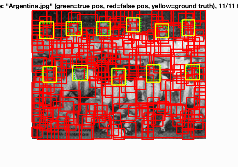
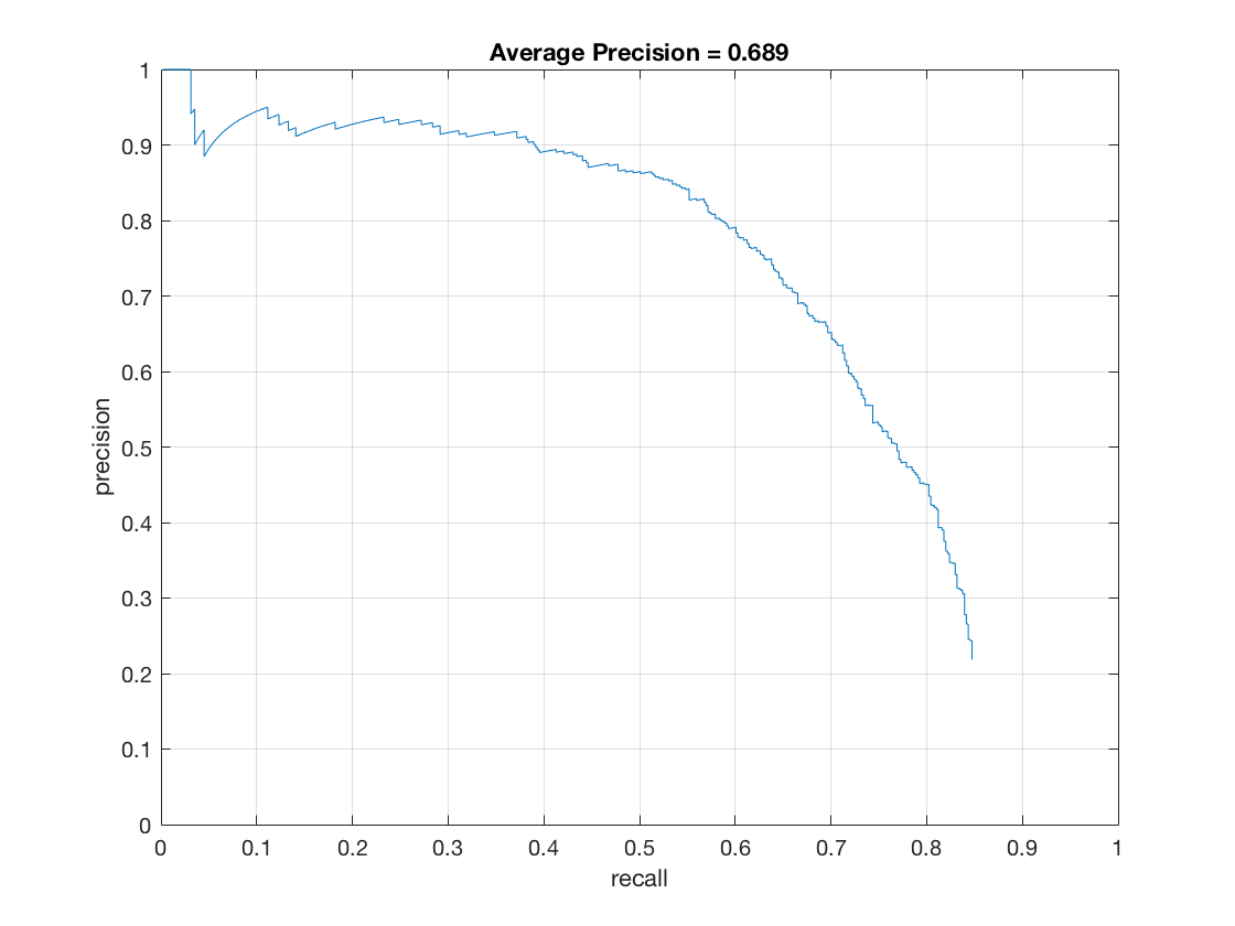
Here are the results with and without sorting the confidences.
Just threshold
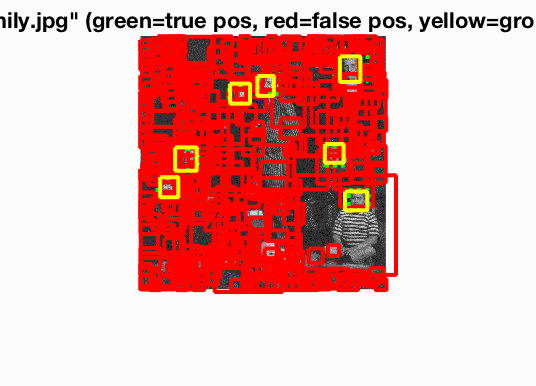
|
Threshold and sort
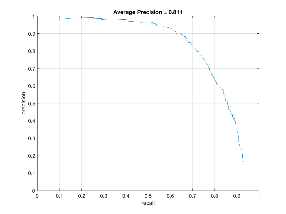
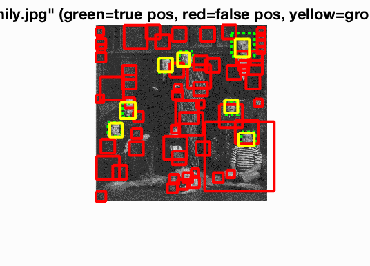
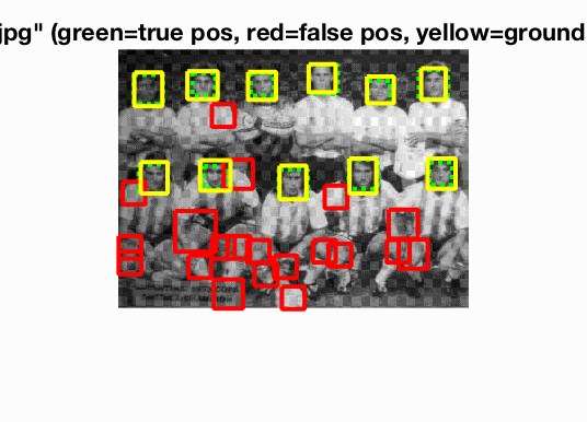
|
Analysis
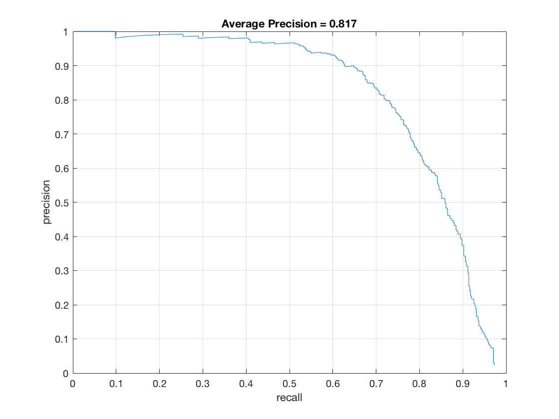
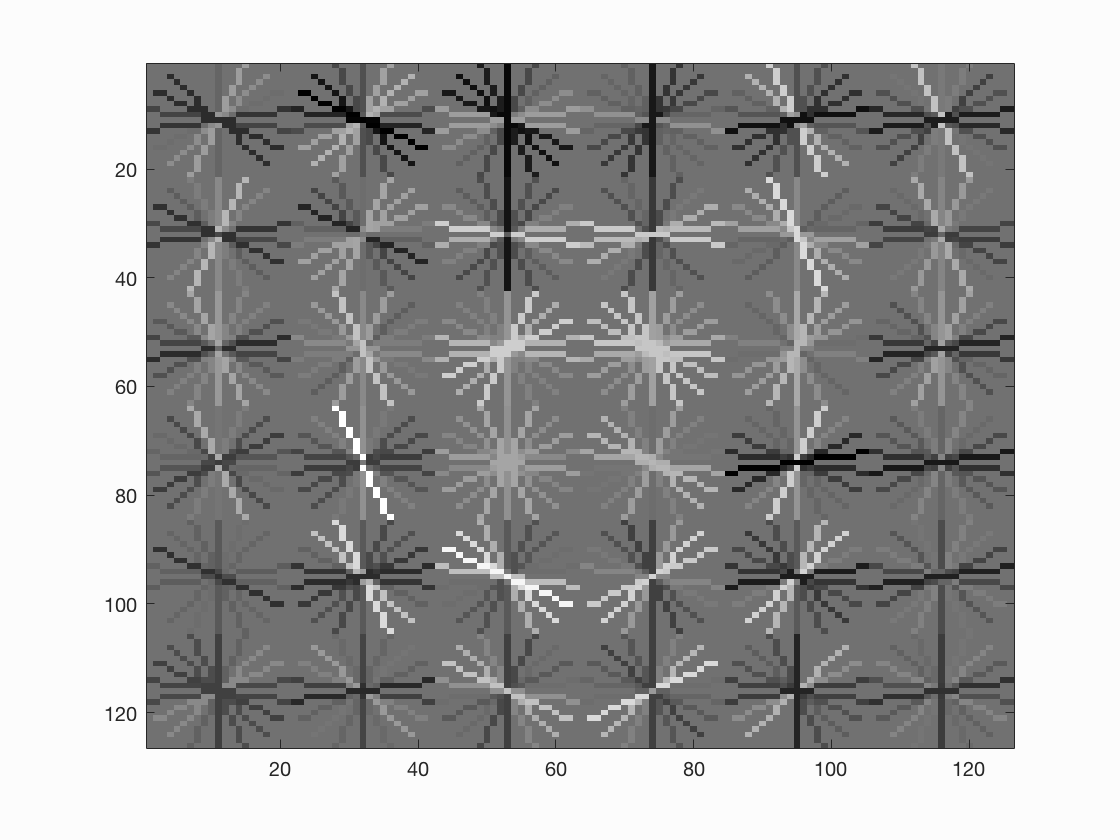
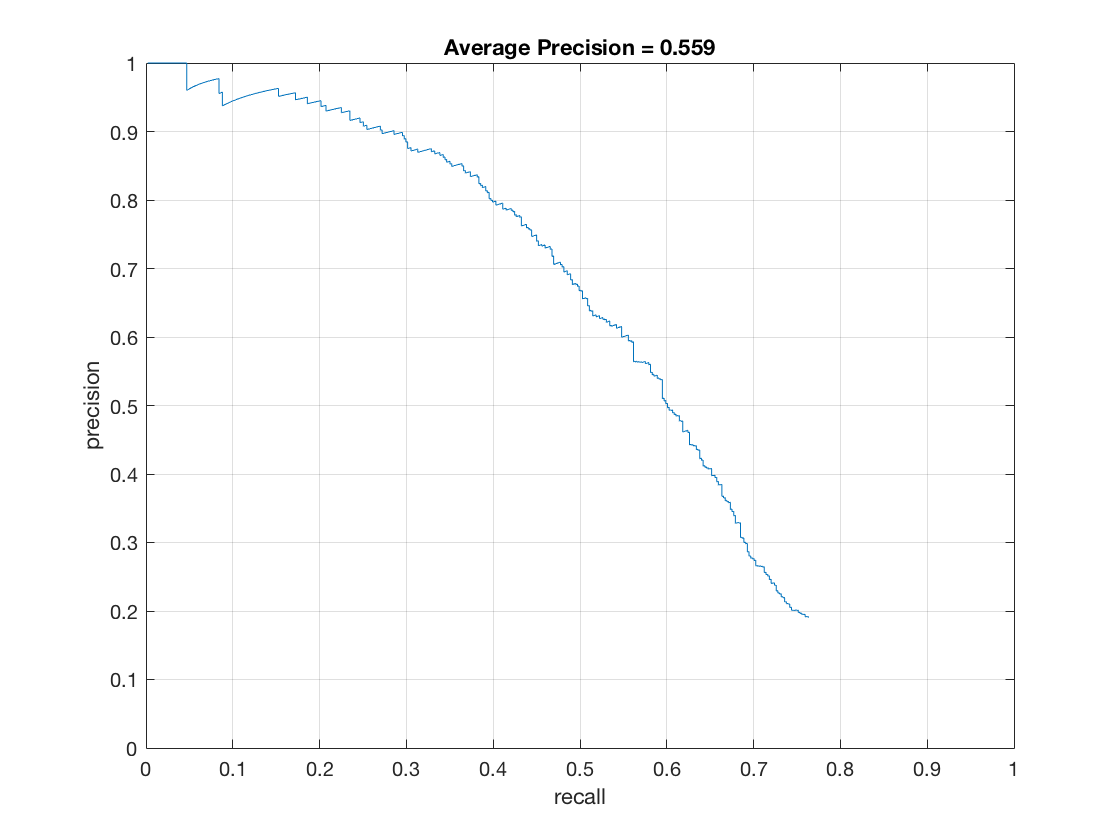
- It's interesting to note that if we visualize the features learnt by the HOG descriptor we see that it looks like a face.
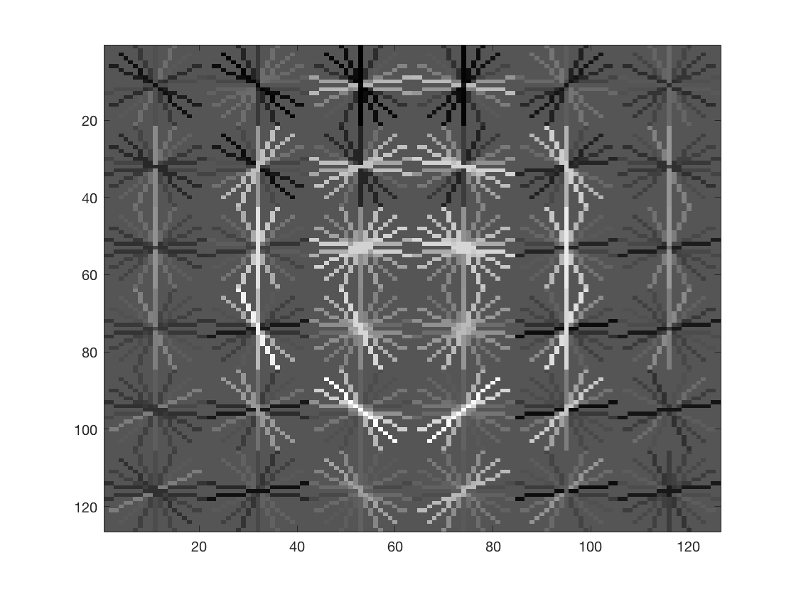
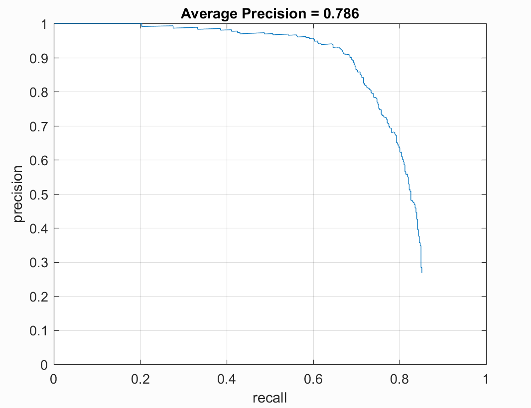
- Without running the detector at multiple scales, the accuracy is only around 40%. Here's the
precision-recall
curve.
-
Effect of cell size on performance. Lowering the cell size increases the runtime and accuracy of the model.
Here's how accuracy varies with cell size:
cell_size = 4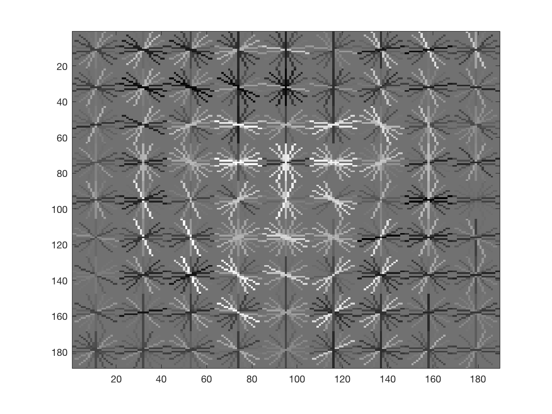
visualisation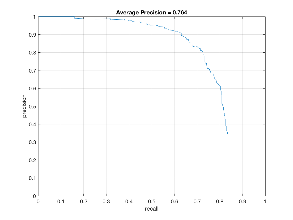
thresh=-2, lambda=0.01
thresh=-2, lambda=0.0001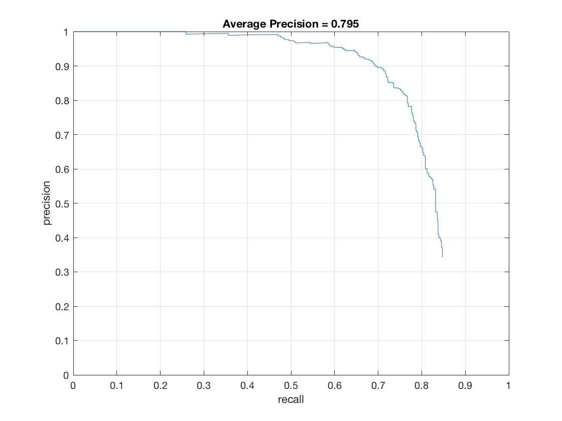
thresh=-0.8, lambda=0.001
cell_size = 2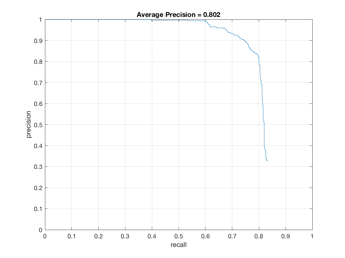
thresh=-1, lambda=0.01
Extra Credit
Hard Mining
In hard mining, we run the detector on the images not containing any faces. We then bolster the negative training images with whatever detections we have obtained above. We then retrain the classifier. Hard mining seems to work very well, but seems to be very sensitive to the threshold. Decreasing the threshold while hard mining and training an SVM classifier with a high lambda makes the model learn to distinguish well between negative and positive images (because higher lambda learns a classifier with a larger margin.
Here's the code for hard mining
        % det_thresh is a very sensitive parameter that affects Hard mining quite a bit.
        [bboxes, confidences, image_ids] = run_detector(non_face_scn_path, w, b, ...
                                            feature_params, true, [1], false, det_thresh);
        % Hard mining is also affected by thresh
        thresh = -0.1;
        for i = 1:numel(image_ids)
            if confidences(i) > thresh
                image_id = image_ids{i};
                img = imread(fullfile(non_face_scn_path, image_id));
                img_crop = single(imcrop(img, [bboxes(i, 1), bboxes(i,2), 35, 35]));
                feat = vl_hog(img_crop, feature_params.hog_cell_size);
                features_neg = [features_neg; reshape(feat, 1, [])];
            end
        end
        Y = [ones(1,size(features_pos, 1)) -1 * ones(1,size(features_neg, 1))];
        X = [features_pos' features_neg'];
        % Setting a high value of lambda gives better results for hard mining.
        lambda = 0.01;
        [w, b] = vl_svmtrain(X, Y, lambda);
Analysis
- Effect of threshold (thresh in code) on hard mining:

thresh = -1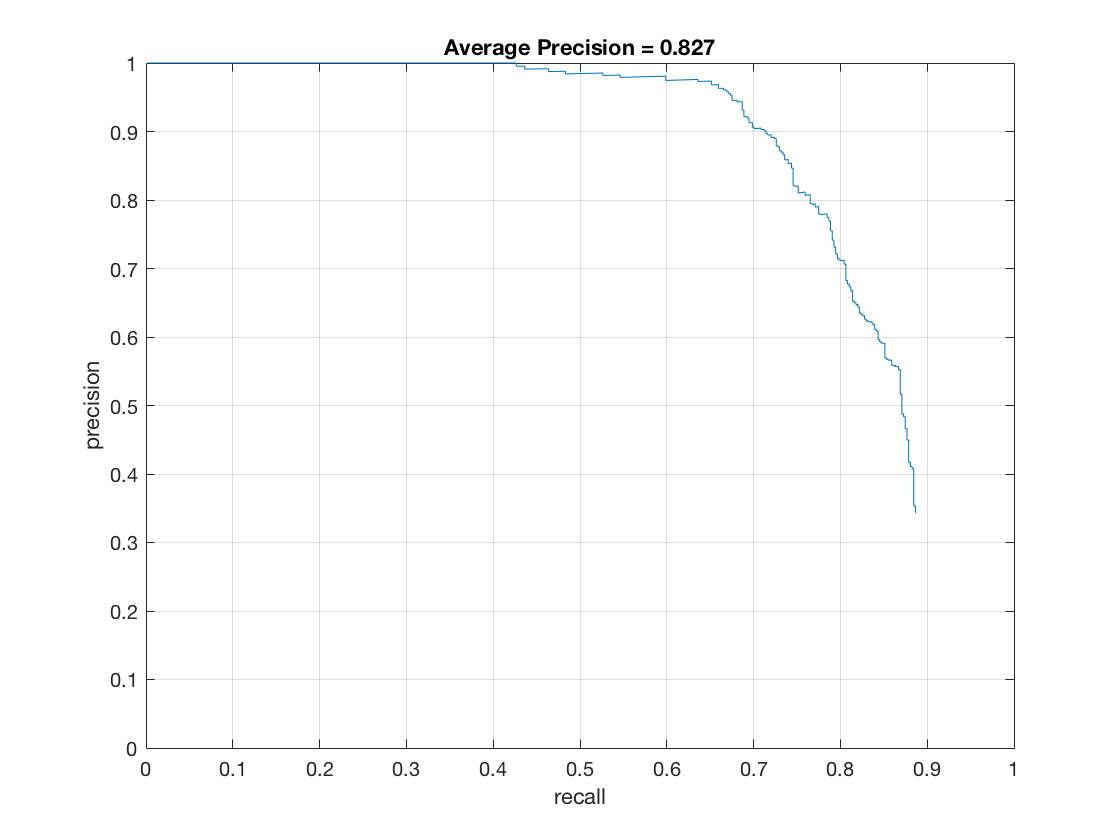
thresh = -0.1
thresh = -1 - Effect of detector threshold (det_thresh in code) on hard mining:

thresh = -4
thresh = -2
thresh = 0 - Effect of lambda on hard mining:
thresh = 0.1
thresh = 0.001
Extra images
I used the data set from LFW database. The problem with using the images directly to bolster the positive images already given to us (Caltech database) was that the face images from the two databases looked completely different. It would have been possible to crop the images from the new database to the correct proportions but it would take too long to crop every image.
Instead I used the fact that the faces in the new image are centered in the image. Using this as the base idea, I used a crude version of active learning to automatically crop the images. I first trained my model on the images present in the Caltech database. Using this model, I ran the run_detector to detect faces in the LFW database images. Knowing that the faces lie around the center of the image, I filtered the detections by
- first taking the larges bounding box found in the image. I realized that this was more likely to be a face compared to other images, especially given that I'm training them on smaller scales, and given that the faces are relatively straight forward.
- then, I compared the centers of the detected bounding boxes with the centers of the images and discarded any bounding boxes lying more than 20pixels away from the center of the image.
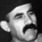
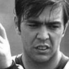
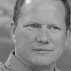
Doing so gave me very good faces. I tweaked the scales at which I detected the boxes and the cropping region around the bounding boxes to get the following faces.

|
I extended this idea even further. I realized that most of the bounding boxes which were not near the center and not the biggest bounding box detected for that image would most likely not be faces, but were still recognized as faces. I could use these images for hard mining given that these images are more closer to actual faces compared to the images extracted from hard mining images not containing any faces. Training the SVM with these faces added to negative images along with a high lambda would theoretically give me a much better accuracy. To be on the safe side, I increased the margin for boxes to be classified as away from the center. Here are some of the 'faces' I obtained from hard mining.

|
Note: To obtain extra faces, run crop_faces.m first. There are two changeable parameters at the top of this
file - use_vl_hog and use_hard_mining. I wouldn't recommend changing
use_vl_hog from its value of true unless you don't mind waiting a few hours to run
the code with my own hog implementation. Setting use_hard_mining to true extracts
'negative faces' from the LFW database.
To augment the positive features with features from the LFW database, set augment_pos_data to
true.
I have also included code to use the extra negative features obtained above for hard mining. This
can be run by setting use_vl_hog = 'mod' in proj5.m.
To be fair, some of these images still do contain faces in them, but that can be easily modified by tuning the parameters for hard mining (like margin, threshold etc.)
Here are the results with extra faces bolstering the positive images:
The low accuracy can be attributed to the fact that the images I extracted from the LFW database are still different from the Caltech database faces. This can be seen from the hog visualization obtained from the model trained on the augmented features:
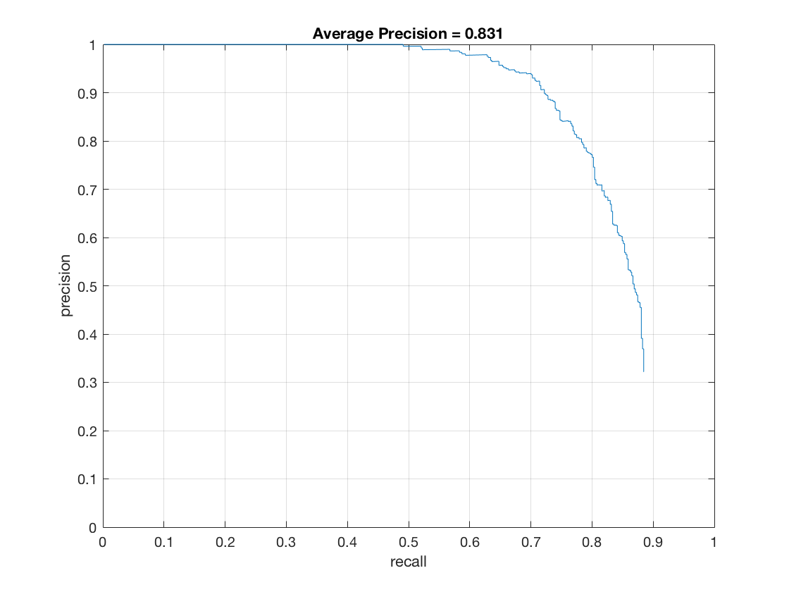
As one can see, this image is quite different from the visualization shown above. This visualization seems to include the top of ones head and some region above it too. This is also one of the reasons why the average precision is so low. With proper tweaking, I was able to obtain an accuracy of 83%. But I didn't save that model, and now haven't been able to reproduce the results. One way to include tuning as part of the model would be to extract hog features from the Caltech database and hog features from the LFW database separately. We can then compare the hog visualizations of the two databases (again, there are different ways to compare them, but I would start with a simple euclidean distance between the two images and go from there) and do a grid search on the hyperparameters for crop_faces.m until we get similar visualizations. These are just ideas to do improve active learning for images without using deep learning (which would require a lot of data). As can be seen, even a simplistic first version prototype performs decently well. Bound by the time constraints of the assignment, I was unable to improve upon my model, or implement the above mentioned idea.
As mentioned above, by hard mining the faces obtained from the LFW database, there is a stark increase in the accuracy (13%!). This can be attributed to the fact that these negative features are obtained by running the detector on actual faces rather than images not containing faces. Despite there being faces in the hard mined negative features, the accuracy of the model improves quite a bit. Tweaking the model would result in much better performance. I will take some time after the assignment is finished to tweak the model, and submit my results, purely in interest of research
Here is the precision-recall curve with hard mining enabled:
Remember to set use_hard_mining to 'mod' to run it in the above mentioned mode.
I also included code to replace the Caltech database with faces obtained from the LFW database as source for
positive images. This can be run by setting < replace_pos_data > equal to < true > in proj5.m. Since this
didn't give me much difference from augmenting positive features, I haven't included the results in the
report. I have also included code to use the extra negative features obtained above for hard mining. This
can be run by setting use_hard_mining = 'mod' in proj5.m.
Building a HOG feature extractor
The HOG feature descriptor is a very simplistic feature extractor that is very similar to the SIFT features. I implemented the HOG feature descriptor given in the Dalal and Triggs paper. The algorithm for it is:
- Divide the image into hxh blocks.
- Extract gradients and magnitudes (sqrt(gx^2 + gy^2)) from each block.
- Bin the gradient angles into n bins weighted by corresponding magnitudes.
- Smooth the obtained histograms by bilinear interpolation.
- Do local contrast normalization. This is done as follows:
- For each hog cell, take the m neighboring cells, and normalize the entire block.
- Depending on m, each hog cell gets m contributions from m possible neighbors.
- All contributions are just appended together to obtain the final descriptor.
Note:The amount of overlap is discussed in the Dalal Triggs paper. They observe that a complete overlap only leads to around 4% increase in the accuracy. Given this fact, and the fact that my HOG implementation is very slow, I trained my model using no overlap even though I implemented complete overlap model too.
Here are the results using my HOG descriptor.
The hog feature visualization:

The precision-recall curve:

To run my hog feature extractor instead of vl_hog, set use_vl_hog = false in proj5
.m
Other features
Given that neural networks perform very well at image classification/recognition tasks, I decided to use a neural network to extract extra features. Given that I was only using it as a tool to extract features, I used a pre-trained network - the VGG-Face implemented in the matconvnet toolbox in vlfeat.
It has to be noted that Matlab doesn't play well with MacOS. I had a lot of difficulty trying to use matconvnet on my system, but Matlab kept complaining about lack of supported compilers on my system even though I installed Xcode 7.0 specifically for this purpose. Apparently older Matlab versions also had an issue with not recognizing the system compiler on MacOS. There were patches for Matlab upto versions 2015b. But I wasn't able to find a patch for v2016a. Given that Matlab R2016b isn't yet available on oit.software .gatech.edu, I had no other way to run matconvnet on my MacOS.
As a result, I had to install a virtual machine running Windows 10 on my system. The first time you try to install matconvnet, Matlab asks to install a supported C++ compiler on the system. Given that they recommend installing mingw as the C++ compiler, I went ahead and did that, only to realise that mingw comes with gcc and Matlab/vlfeat looks for cl.exe (which is Microsoft Visual Studio's supplied compiler of C++). The resulting model also runs extremely slowly given that it runs on a virtual machine and that a virtual machine has no access to the system GPU. The runtime becomes approximately 10 times the runtime of the baseline model even without training the model.
Long story short, installing matconvnet is a very tiring and long process that is especially complicated by the fact that Matlab keeps misleading us with it's recommendations. As such, even though the remaining code written by me works on MacOS, the part requiring matconvnet will only run on a windows system with a visual studio C++ compiler installed and accordingly set up in mexopts.
After installing matconvnet, I used the pre-trained VGG-Face net as an extra layer of classification. That is, I would first get detections using HOG, suppress them using non-max suppression, and then I would pass the remaining boxes to VGG-Face to be classified as face/not face.
An inspection of the layer meta properties of VGG-Face net reveals that it has been trained on images of size 224x224x3. This can be taken care of by just extracting the features from the last convolutional layer. But passing in images of much less size and quality only give bad features. The VGG-Face net classifies most of the non faces as not faces but also misclassifies some faces as not faces, thereby reducing the average precision of the entire pipeline.
Here are the results of that:
Other classifiers
Since the VGG-Face net was performing badly, I decided to train a neural network from scratch with the given images. Given that matconvnet performs extremely on my system, I decided to implement the neural network in python (I asked if it was okay to do that on Piazza, and instructor Varun Agarwal replied in the affirmative).
On a side note, I tried quite hard to run the resulting python pipeline from Matlab code. Matlab does make it possible to run some (quite few actually) functions from python. It alsow allows users to define python modules in the Matlab project, and call them from Matlab as one would call normal Matlab functions. Both of these features make use of inbuilt Matlab wrappers for a few python functions. Given that I was trying to build a neural network, both of these options became invalid for me. Next, Matlab allows a user to run system commands from a Matlab project. But when I tried to run my python code from Matlab, it would either crash my system python or Matlab itself. After sending a crash report to both Matlab and Apple, I had to give up on this route too.
Once again, long story short, after running the first 7 steps in my Matlab proj5.m code, one has to pause, run the supplied python code as mentioned in the proj5.m file, and then once it finishes, come back to Matlab to run the remaining code cells. While I realize that this process is not very intuitive and quite tedious, my main motive was to implement new models and learn how each model interacts/performs with the given data and task. As such, I ask that you kindly consider the model with all it's faults (in terms of ease of use).
I trained quite a few models in Python using keras 1.1.1 with Theano 0.8.2 as the backend. I started with the simplest network - a fully connected network. My reasoning for this was that the images provided are very small and of very low resolution. I thought an fcn would be a decent approximation of a convnet, especially given the small amount of training data. Experimentation seems to solidify this idea. All models I built were quick to reach 100% validation accuracy. Without significantly improving the complexity and non-linearity of the network, the models over-fit the training data very quickly and wouldn't learn much after that.
Here are some of the different models I tried:
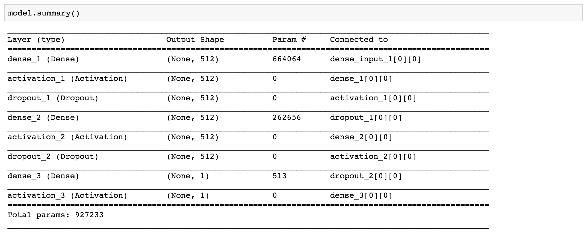
Fully connected feed forward network:
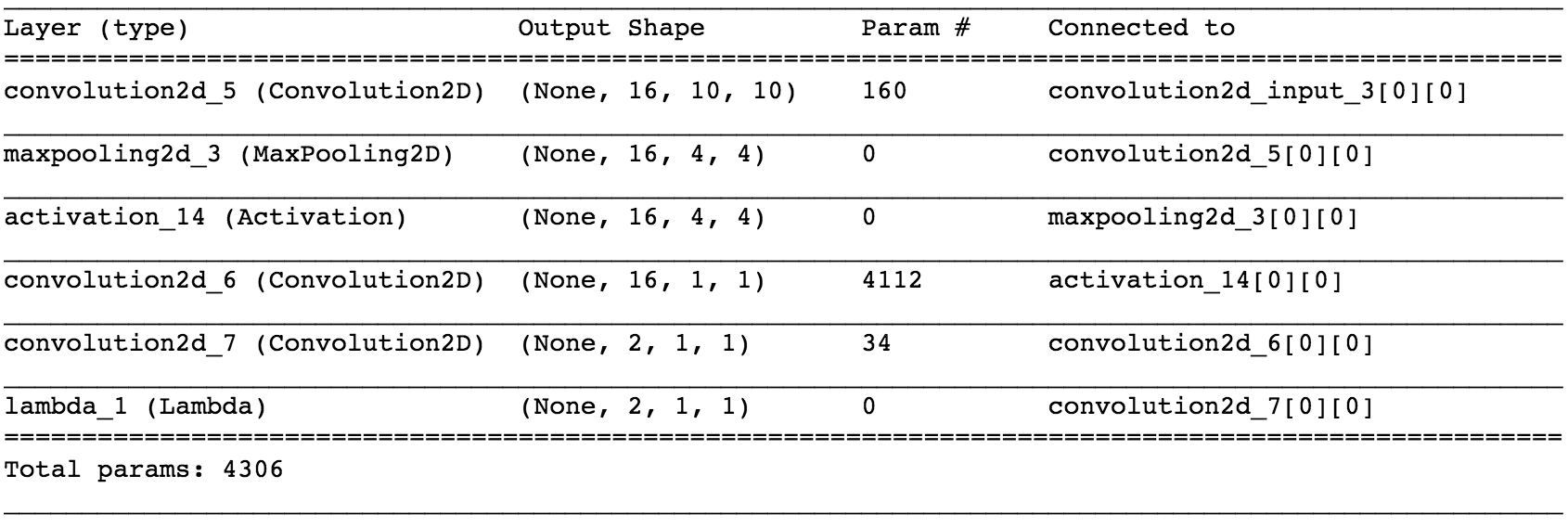
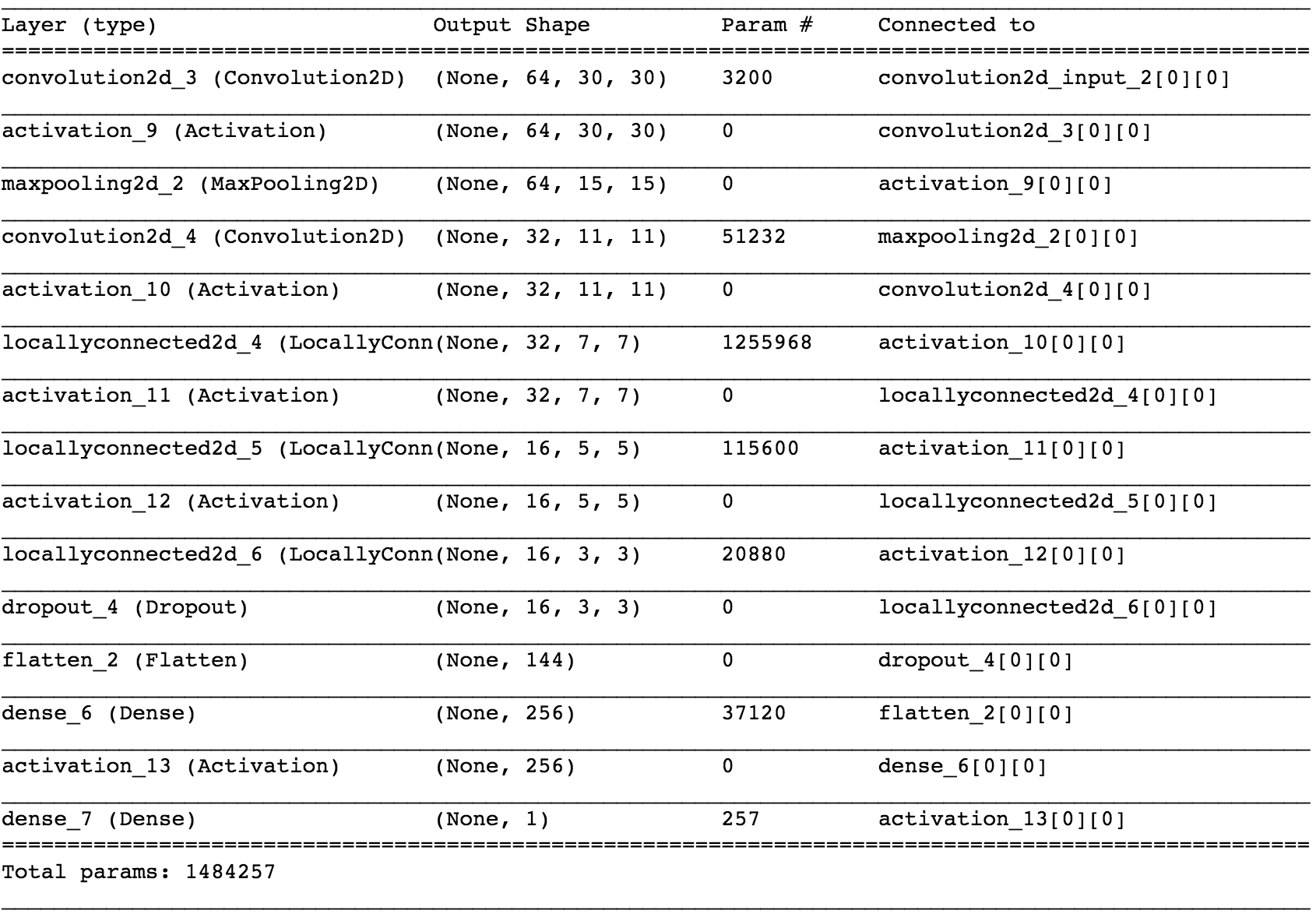
Fully convolutional network:
I also tried out the Deep Face network, without much success. The very limited amount of training data made it very hard to train such a complicated network. Needless to say I obtained no where near the results obtained in the original paper. It didn't even perform as well as my feedforward network!
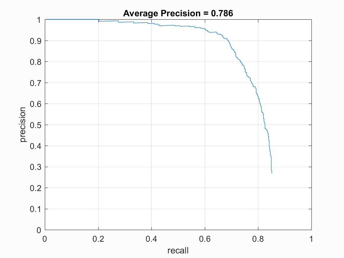
Given that I didn't have much data to train the model on, the model performs decently well. Here is the precision recall curve for the best model I obtained:
One thing to note is that, given the small amount of training data, the inherent randomness in training the training of a neural network gave me widely varying results each time I ran the model despite using a scaled Gaussian initialization for the weights.
To run this part of the model, set use_py_nn = true. And when the program pauses,
do as mentioned in the comments of the code in Step 7. of proj5.m