Agrata Kumar

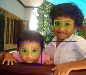
Example of face detection using Haar Cascades.

Feature Extraction for Training the Classifier

In order to train a simple classifier which can classify the faces from non-faces, it should know about the features of both the faces and non-faces. So a feature set (containing the HOG features) was extracted from both the set of both the positive and negative examples. All the positive examples given were cropped to a size of 36X36. vl_hog with a hog cell size of 6 was applied. The negative examples were not of consistent size. For these images a random patch of size 36X36 was first extracted and then vl_hog was applied on it take it to the feature space. The number of patches which were extracted depended on the number of features specified. For the baseline 10,000 features were extracted from the negative dataset.

A simple Linear Classifier

Once the features were extracted, they were fed to a simple Linear SVM in order to get the trained parameters. The SVM is very sensitive to the value of lambda.

Run Detector

After learning the training parametrs, the last step was to use them to detect the faces in the testing dataset. The simple sliding window detector was completed using the starter code. This detector was run for different scales of the image. The scales chosen were 1, 0.9, 0.81, 0.729 and 0.6561. Also, another parameter which can be tuned is the threshold used for classfication. It was kept to be a lower value, to make sure that a few detections are made from all the images in the dataset. If the threshold value was increased then nothing was being detected in the images "aeon1a.jpg" and "bwolen.jpg". But reducing the threshold to a lower value meant many detections in other images. In order to avoid this, the confidences were sorted and a limited number of bounding boxes were picked up from all the detections, based on the size of the image.

Results in a table

First the detector was tested by taking 100000 negative examples and at a single scale. The average precision achieved in this case was 38%. To further improve the results, the detector was run at multiple scales. The scales chosen were [1, 0.9, 0.81, 0.729, 0.6561]. A total of 10000 negative features were taken. After extracting the hog of the entire image, 6X6 boxes were extracted which were used to generate the bounding boxes for the faces with a certain value of confidence. The threshold value of lambda for the classifier, the size of the template and the hog cell size and the threshold value for finding the bounding boxes are the parameters which determines how well does the detector perform.

Value of Lambda	Value of threshold	Accuracy
0.005	-2	71.70%
0.005	-6	71.50%
0.001	-3	71.3%
0.003	-3	72.10%
0.005	-3	73.20%
0.006	-3	71.90%
0.01	-3	70.90%

Extra Credit

Additional Dataset

Mirror Images

Before proceeding further, the positive faces dataset was made more robust by adding the mirror image of the faces in the dataset. So now instead of having just 6713 positive examples, the classifier was trained on 13426 positive images. This did not improve the accuracy. The average precision achieved was 71.2% using the same parametrs as mentioned above for the best results.

LFW Dataset

The LFW dataset was downloaded. The faces were not of the size of the cropped faces provided. But it was observed that the faces were centred and so a bounding box from the centre of the image was cut to have a face in it to be of the same size as. These cropped faces were then added to the dataset of the original Caltech Cropped faces dataset and the results were analyzed. Only one image for each person was taken. By just adding this to the positive dataset, the average precision with lambda of 0.0001 decreased to 64.7%. By using the lamda of 0.0005 it was improved a little to 71.1%, but with a value 0.0009 that it was reduced back to 64.3%

The positive dataset was created by adding the features extracted from the given dataset, the dataset obtained by taking the mirror images of the same and the faces extracted from the lfw dataset. The results were recorded for different values of lambda.

Value of Lambda	Value of threshold	Accuracy
0.005	-3	72.20%
0.0055	-3	69.8%
0.0052	-3	71.2%

Hard Negative Mining

The training in the baseline was done by taking the positive images and randomly selected crops of same size (as that of the positive images) from the negative images and passing them through a classifier to get the training parameters. To refine the classifier the detector was run on the negative examples and all the crops which were falsely classified as faces were added to the negative dataset and the classifier was retrained using this new negative dataset. This step was repeated multiple times with the different values of lambda and the results were recorded.

Value of Lambda	Value of threshold	Accuracy
0.004	-3	72.30%
0.005	-3	73.70%
0.006	-3	70.80%

This table shows the result of hard mining by just using the base dataset, at 5 scales. The dataset consisted of the positive and their mirror images and the negative image dataset.

The positive dataset used for the negative mining consisted of the given positive images, their mirror images and the faces added from the LFW dataset. The result was recorded for the lambda of 0.005. The avaerage precision obtained was 71.1%. I was expecting it to improve but it did not drastically improve.

Combinations of different features

With the HOG features, the GIST features were also added to both the negative and positive feature dataset. But this took very long to run, about 12-13 hours. Tested it for one scale and for a reduced dataset. The average precision instead of increasing reduced to 61.3%. This can be baucause the GIST feature do not give the local information.

The Figure showing the HOG Template

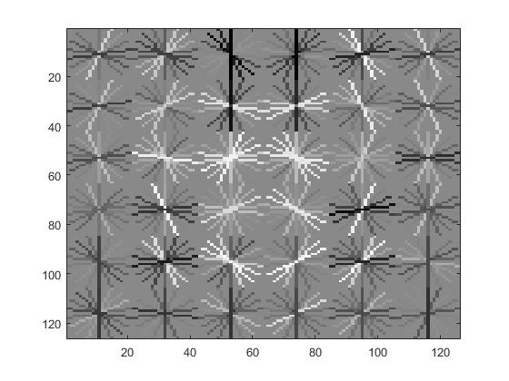
The figure showing the average precision achieved using the value of lambda 0.005 and threshold -3. The best result obtained by using 5 scales of the image and the hog cell size of 6.

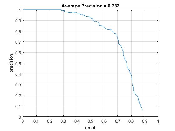
Example of detection on the test set.

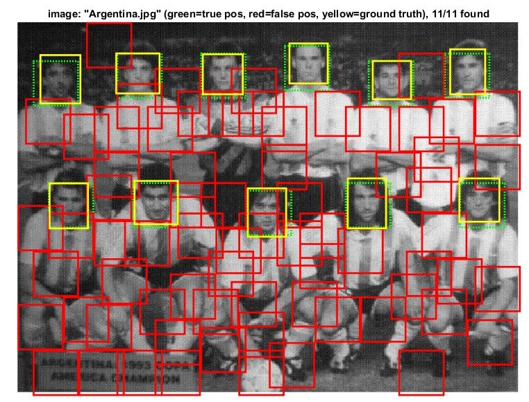
Conclusion

The face detection system using the sliding window was developed. The accurcy achieve was approximately 74%.