Project 5 / Face Detection with a Sliding Window
Table of Contents:
- Motivation
- Project Outline
- Get_Positive_Features
- Get_Random_Negative_Features
- Classifier Training
- Run Detector
- Graduate Extra Credit
- Conclusion
- Sources
Motivation:
The sliding window plays an integral role in object classification, as it allows us to localize exactly where in an image an object resides. A sliding window is a rectangular space of fixed height and width that slides across an image. A visualization of the process is as follows:
The sliding window will effectively allow us to independently classify all image patches as being object or non-object. For face classification, the sliding winow is one of the most noticeable successes of computer vision. Navneet Dalal and Bill Triggs' Histograms of Orineted Gradients for Human Detection outlines a simple but effective algorithm for face detection using a sliding window. Dalal-Triggs focues on representation more than learning and introduces the SIFT-like Histogram of Gradients (HoG) representation. The feature extraction and object detection pipeline that Dalal-Triggs introduced is as follows:
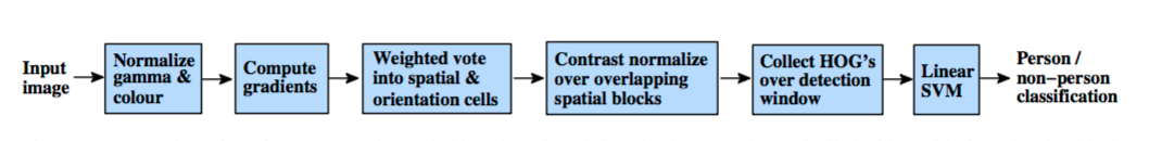
Let us quickly overview this pipeline:
- The detector window is tiled with a grid of overlapping blocks in which Histogram of Oriented Gradient feature vectors are extracted.
- The combined vectors are fed to a lienar SVM for object/non-object classification.
- The detection window is scanned across the image at all positions and scales.
- Non-maximum suppression is run on the output pyramid to detect object instances.
Project Outline:
In our past projects we have implemented a SIFT descriptor, and thus we will not implement the SIFT-like Histogram of Gradients representation. However, we will implent the rest of the pipeline: handling heterogenous training and testing data, training a linear classifier (a HoG template), and using our classifier to classify millions of sliding windows at multiple scales.
Our project will consist of the following matlab files:
- proj5.m: The top level script for training and testing our object detector.
- get_positive_features.m: A file we will implement that loads cropped positive trained examples (faces) and converts them to HoG features with a call to vl_hog.
- get_random_negative_features.m: A file we will implement that samples random negative images from scenes which contain no faces and converts them to HoG features.
- classifier_training: A file we will implement that trains a linear classifier from the positive and negative examples with a call to vl_trainsvm.
- run_detector.m: A file we wil implement that runs the classifier on the test set. For each image, the classifier will run at multiple scales and then call non_max_supr_bbox to remove duplicate detections.
- evaluate_detections.m: Computes ROC curve, precision-recall curve, and average precision.
- visualize_detections_by_image.m :Visualize detections in each image. We can use visualize_detections_by_image_no_get.m for test cases which have no ground truth annotations (e.g. the class photos in the data directory).
- Extra Credit: We will additionally implement variations of the files above for our extra credit. We will describe these in more detail in the extra credit section.
Let us run proj5.m without any implementation and observe the initial results:
Initial classifier performance on train data:
accuracy: 0.500
true positive rate: 0.500
false positive rate: 0.500
true negative rate: 0.000
false negative rate: 0.000
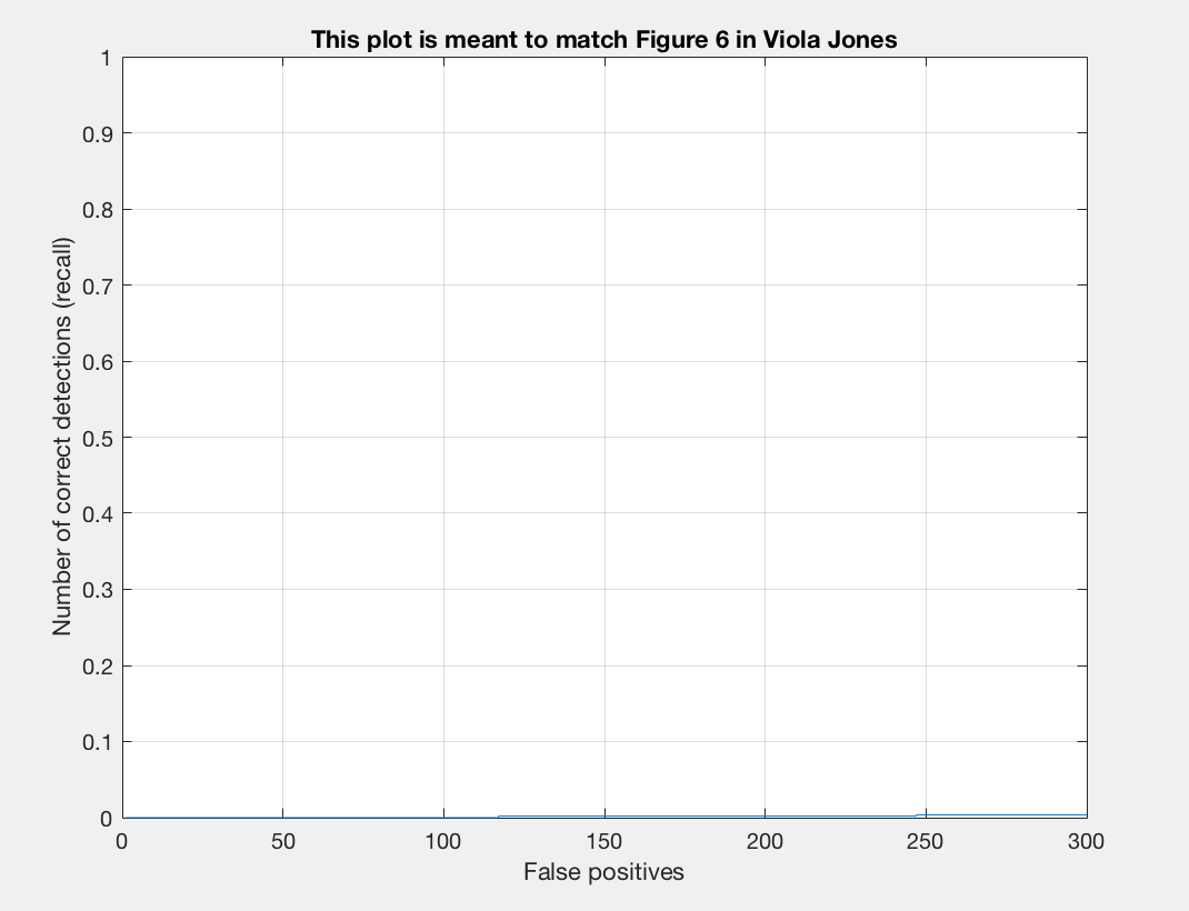
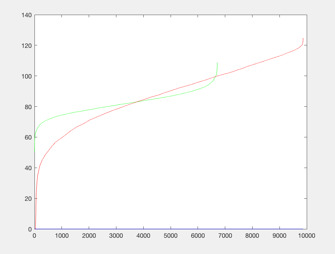
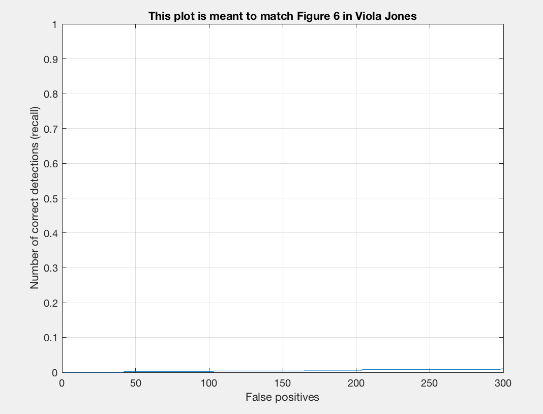
 Precision/Recall |
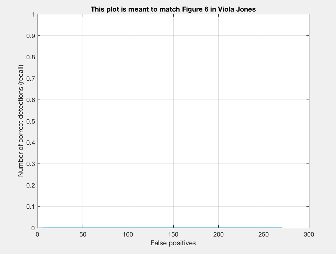
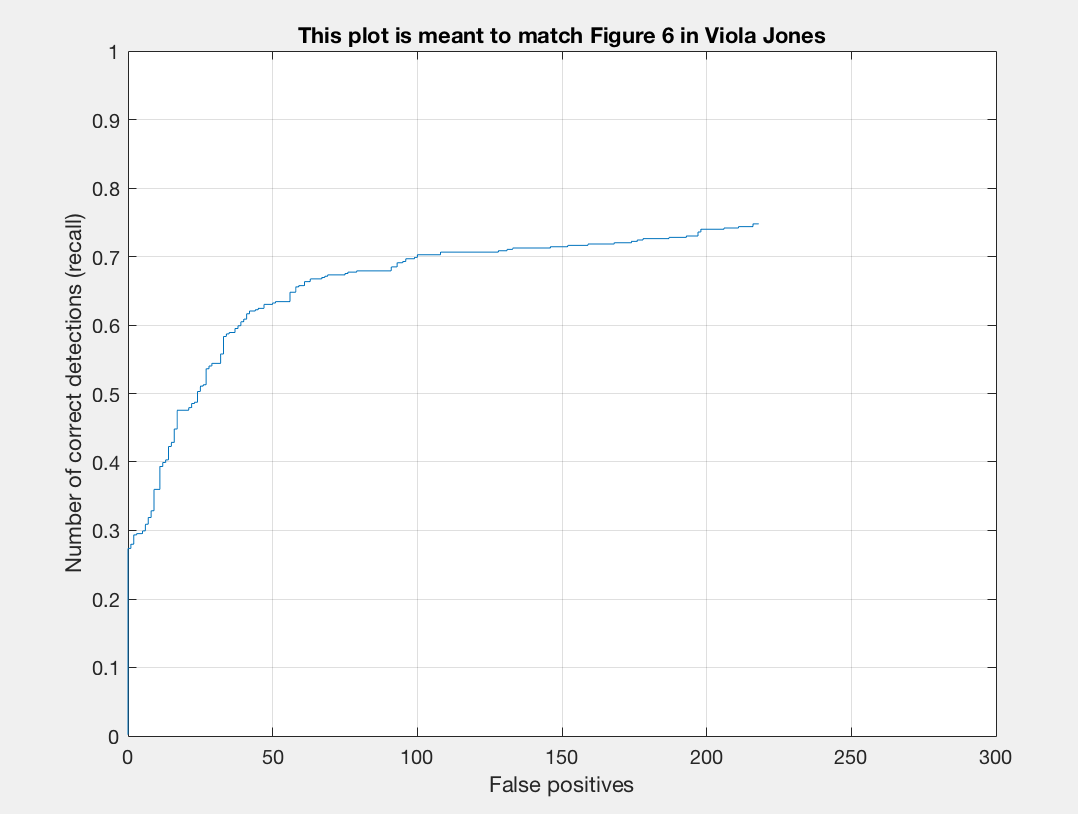
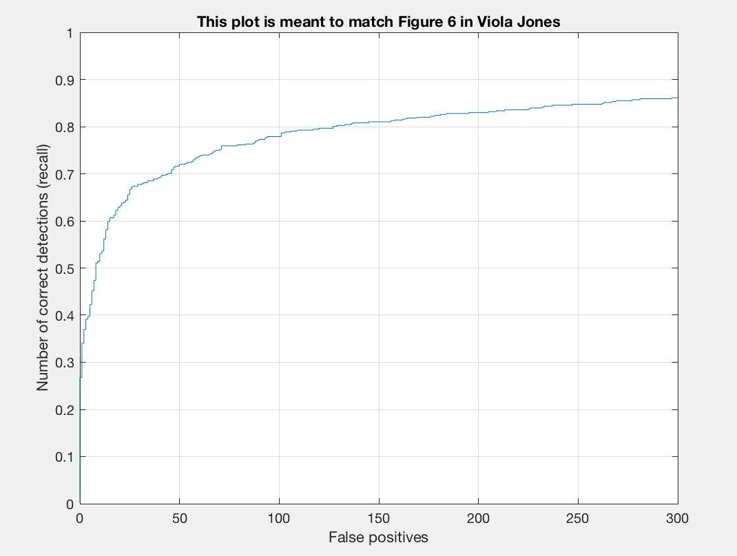
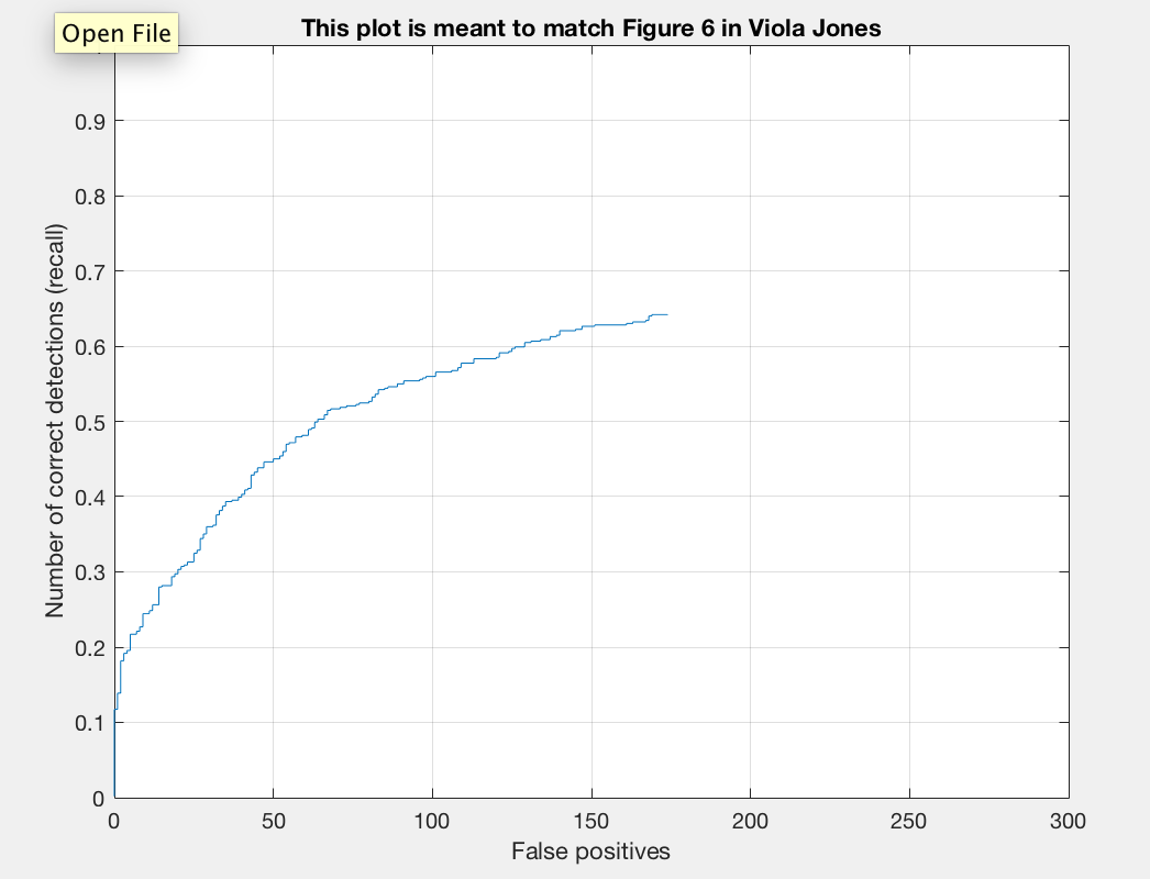
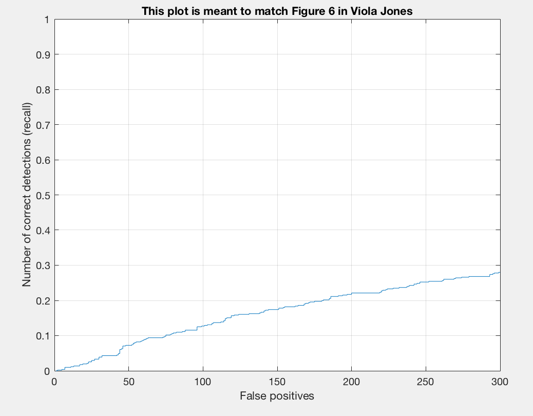
 Recall/False Positives |
 P3 |
|---|
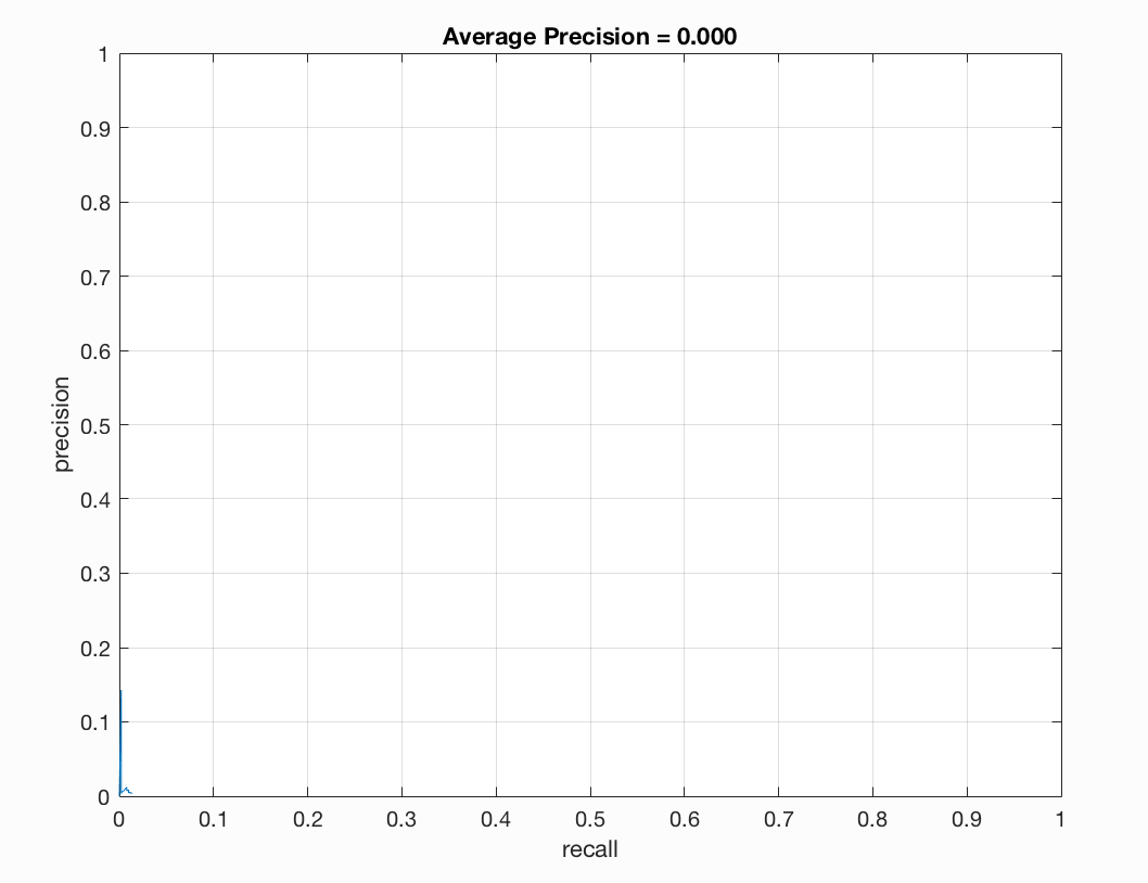
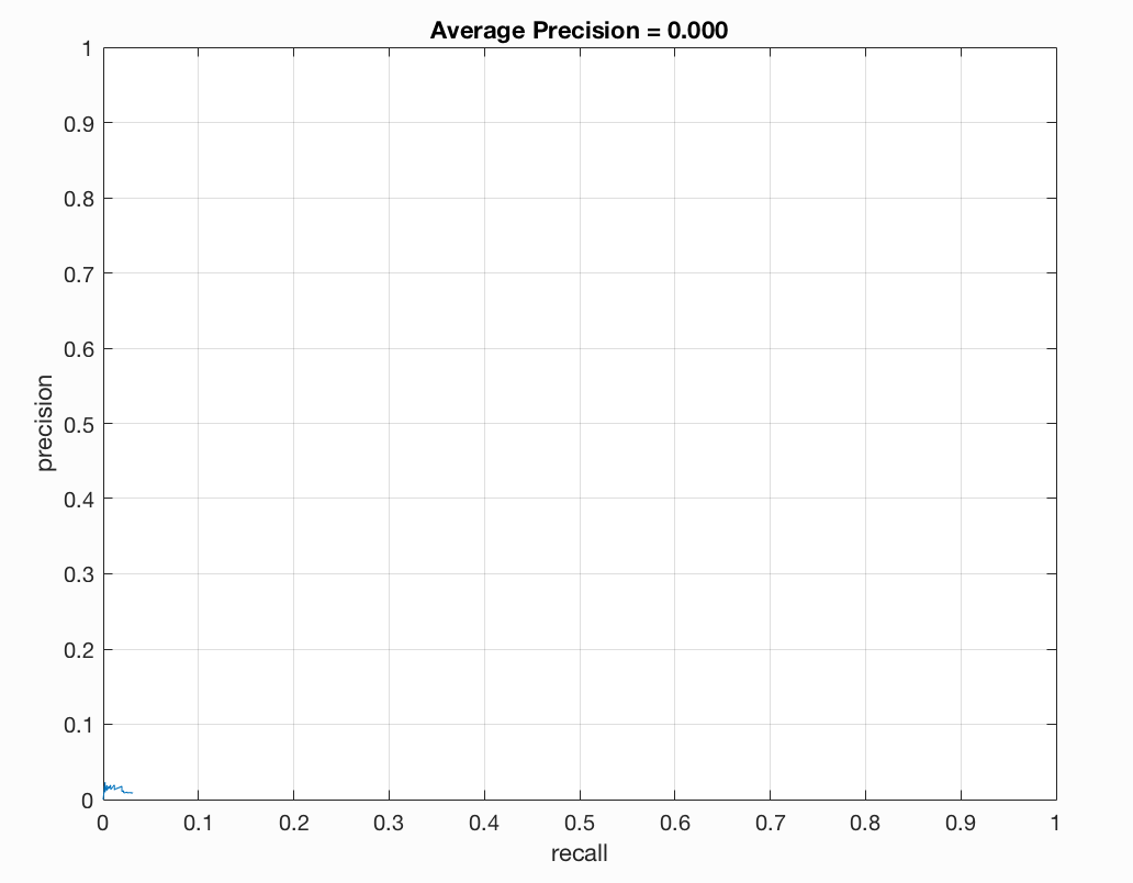
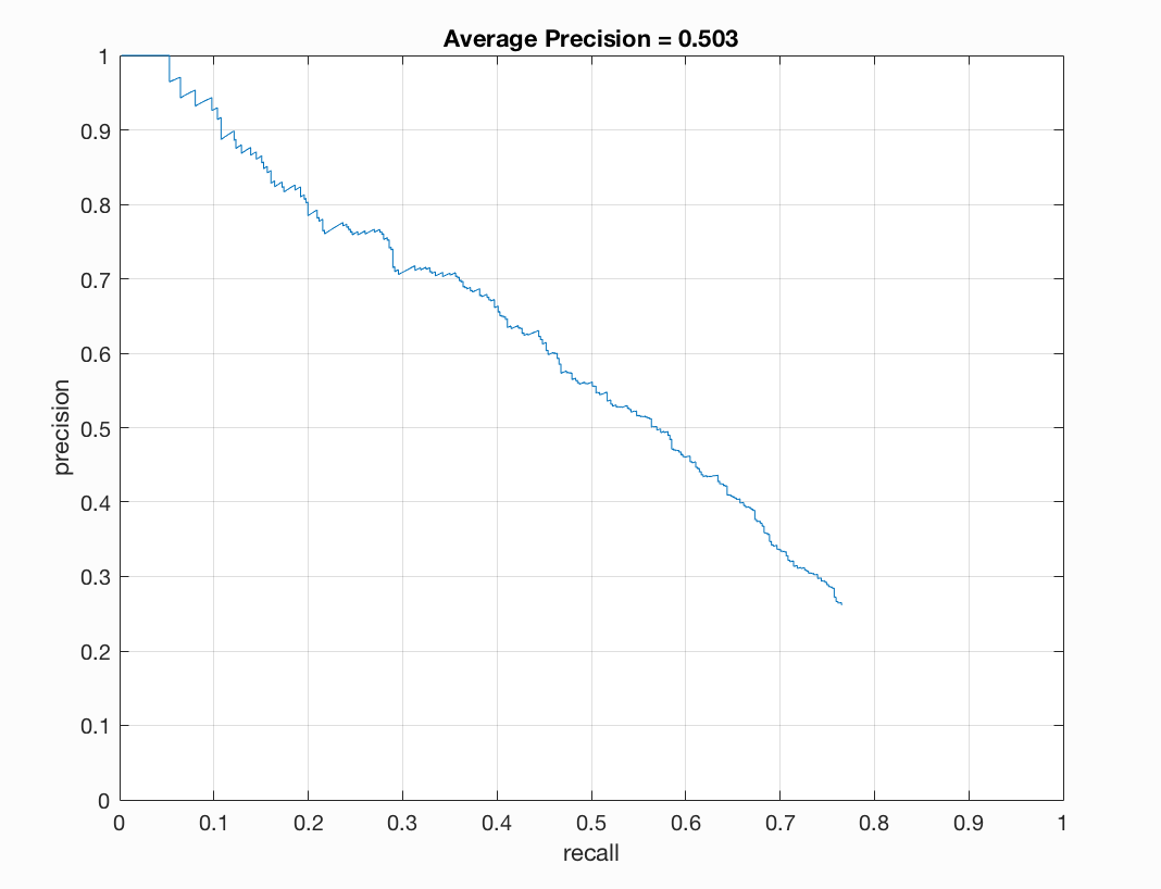
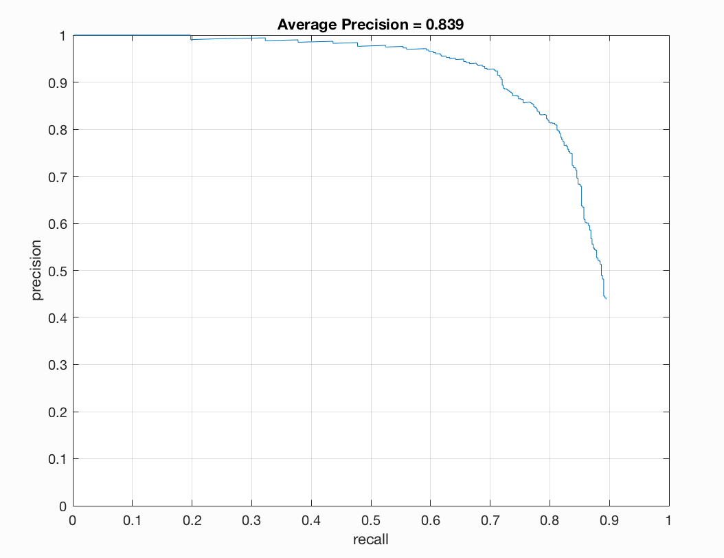
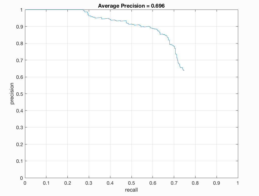
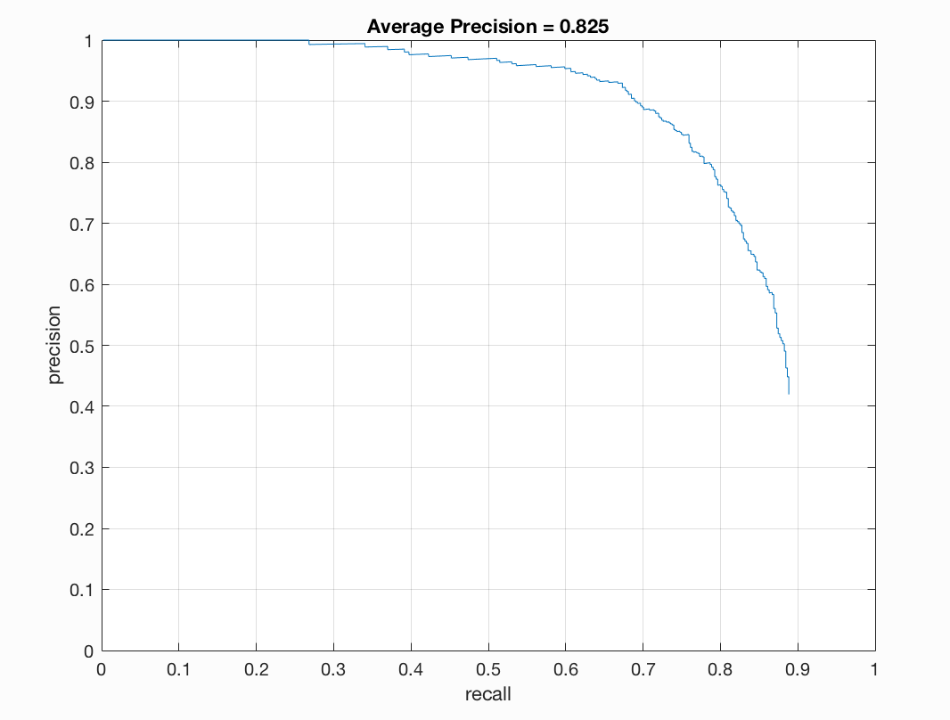
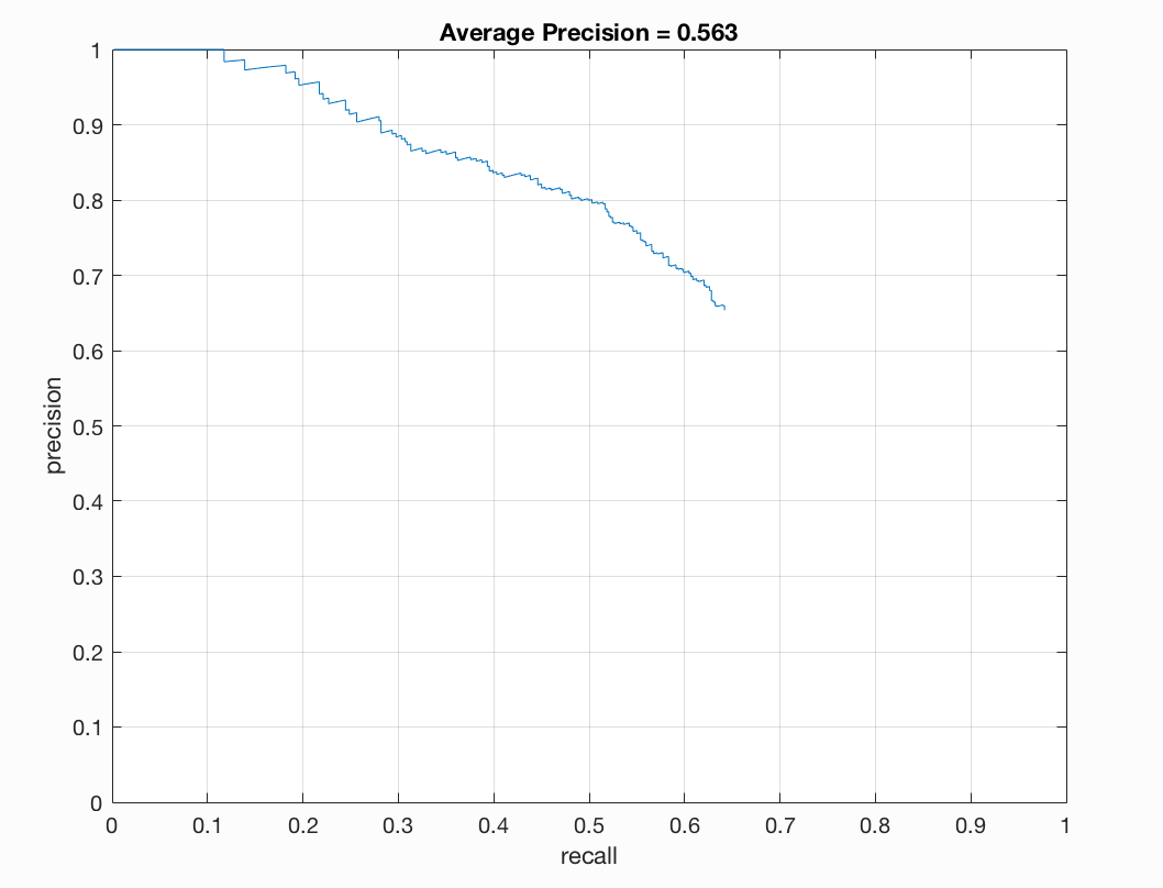
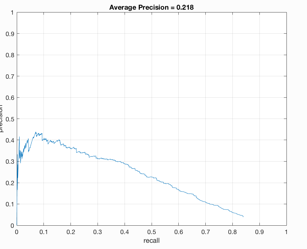
The Precision/Recall chart is a chart that plots precision versus recall. Precision is the fraction of retrieved instances that are relevant, while recall is the fraction of retrieved instances that are retrieved. We can quantify precision and recall as follows:
$$\text{Precision} = \frac{\text{true positives}}{\text{true positives + false positives}}$$
$$\text{Recall} = \frac{\text{true positives}}{\text{true positives + false negatives}}$$
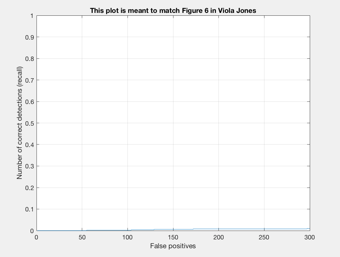
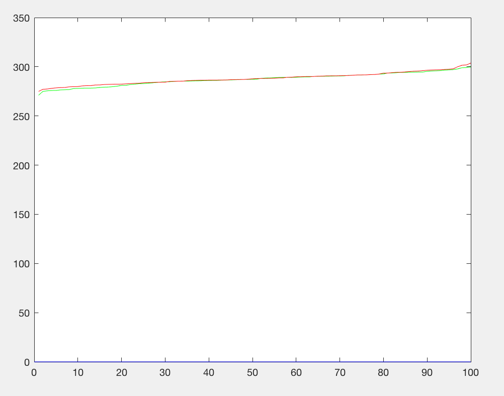
The trade-off between precision and recall can be observed using a precision-recall curve.
In our precision-recall curve we see that we have a small line because a random detector is a poor choice. It is very difficult to randomly guess face locations, unlike secene classification which has a $\frac{1}{15}\sim 7\%$ chance. So, precision and recall are very low. Looking at our results we see that the average precision is basically 0.000. This is to be expected though as we have not implemented any testing details.
Let us now implement get_positive_features.m and see how our training data statistics change.
Get_Positive_Features:
This function will return all positive training examples (faces) from 36x36 images in 'train_path_pos'. Each face will be converted into a HoG template according to 'feature_params'.
- Parameters:
- train_path_pos :A string. This dictionary contains 36x36 images of faces.
- feature_params :A struct with fields feature_params.template_size (defaults to 36), the number of pixels spanned by each train/test template, and feature_params.hog_cell_size (defaults to 6), which is the number of pixels in each HoG cell.
- Output:
- features_pos :An N by D matrix where N is the number of faces and D is the template dimensionality, which would be (feature_params.template_size / feature_params.hog_cell_size)^2 * 31 if you're using the default vl_hog parameters
- Setup Variables: We let image_files be the directory of the fullfile of train_pos_paths with .jpg. We let num_images be the length of the image_files vector.
- Create features_pos vector :We create a vector of zeros with size(num_images,feature_params.template_size / feature_params.hog_cell_size)^2 * 31). The second parameter in the size vector is our D dimensionality since we will use the vl_hog parameters
- For loop :We iterate over num_images. We first extract the name from image_files of i and then strcat train_path_pos with name. We then read in this variable and turn it to a single data type. We then let f represent our feature_params.hog_cell_size and run vl_hog with parameters our image and f. We then reshape it to a vector of size [1 feature_params.template_size / feature_params.hog_cell_size)^2 * 31] and let features_pos(i,:) equal this vector.
Let us now run proj5.m with the newly improved get_positive_feature.m function. The results are as follows:
Initial classifier performance on train data:
accuracy: 0.985
true positive rate: 0.985
false positive rate: 0.015
true negative rate: 0.000
false negative rate: 0.000
 Precision/Recall |
 Recall/False Positives |
 P3 |
|---|
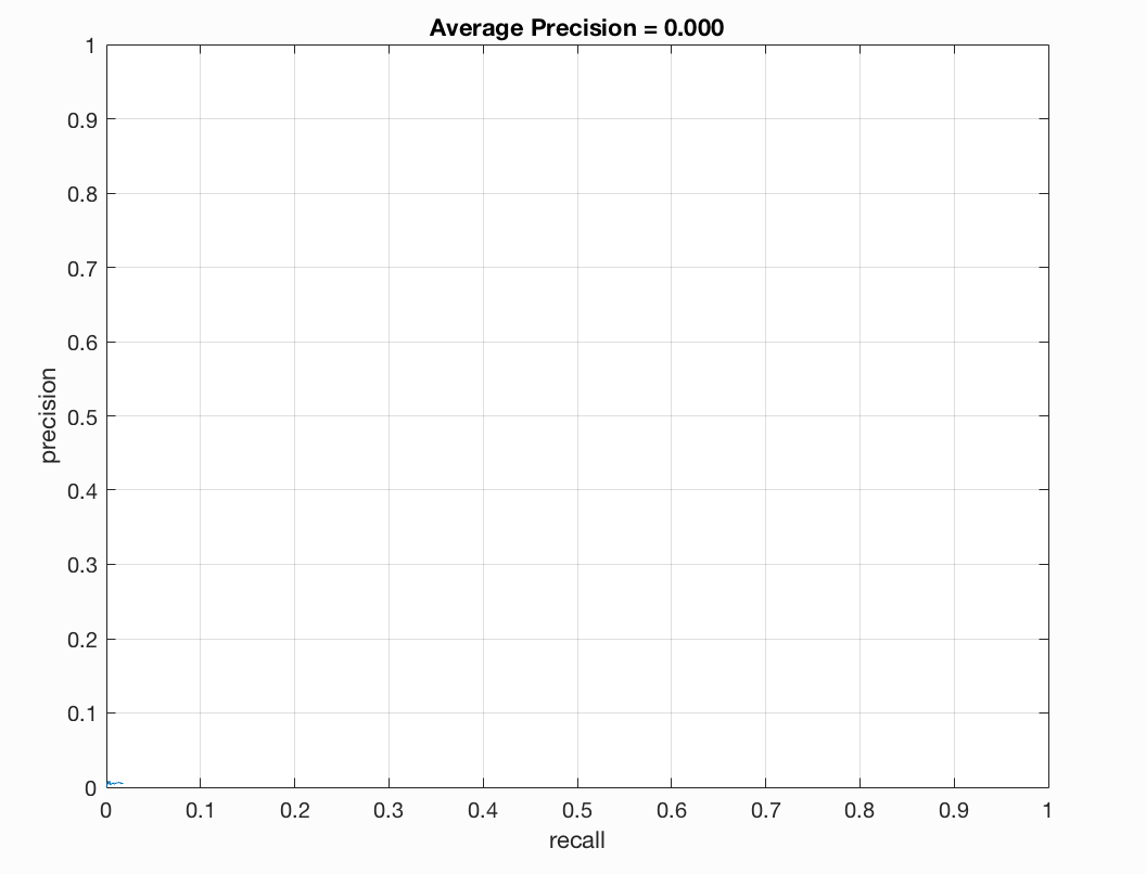
Compared to no implementation, we see that our training accuracy is much better and that our average precision is still 0.000 as we have not implemented any test data testing of our code. We also note that our true positive rate increased and the false positive rate decreased. Our true negative rate and false negative rate remained the same.
Let us now move on to implement get_random_negative_features.m.
Get_Random_Negative_Features:
This function will return negative training examples (non-faces) from any images in 'non_face_scn_path'.
- Parameters:
- non_face_scn_path :A string. This dictionary contains many images which have no faces in them.
- feature_params :A struct with fields feature_params.template_size (defaults to 36), the number of pixels spanned by each train/test template, and feature_params.hog_cell_size (defaults to 6), which is the number of pixels in each HoG cell.
- num_samples: The number of random negatives to be mined.
- Output:
- features_neg :An N by D matrix where N is the number of non-faces and D is the template dimensionality, which would be (feature_params.template_size / feature_params.hog_cell_size)^2 * 31 if you're using the default vl_hog parameters
- Setup Variables: We let image_files be the directory of the fullfile of train_pos_paths with .jpg. We let num_images be the length of the image_files vector.
- features_neg: We create a matrix of zeros that has dimension (num_samples, (feature_params.template_size / feature_params.hog_cell_size)^2 * 31).
- For loop: We iterate over num_images. Outside our loop we have a count variable called idx_count. First we get the name of image_files(i) and store it in a variable called name. We then create a path variable which is imread or strcat of non_face_scn_path + '/' + name. We then take this variable and turn it into grayscale since the positive training data is only available in grayscale. We then turn this into a single datatype using matlab's im2single function and store it in a vairable called img. We then calculate a height variable as size(img,1) and a width variable as size(image,2).
- Nested for loop: We create two random numbers r1 and r2. We let d1 be our width - feature_params.template_size and d2 be height - feature_params.template_size. We then let lx be the ceiling of r1*d1 and ly be the ceiling of r2*d2. lx is the top left x corner and ly is the top left y. We then create lx_eps as lx+feature_params.template_size -1 and ly_eps as ly+feature_params.template_size-1. We then create a variable called box_img which is our img(ly:ly_eps, lx:lx_eps). We then run vl_hog on our image with feature_params.hog_cell_size and reshape this into a vector of size [1 (feature_params.template_size / feature_params.hog_cell_size)^2 * 31]. We finally append this into features_neg at row idx_count. We then add 1 to idx_count.
- Take indices: We finally let features_neg = features_neg(1:idx_count,:).
Let us now run proj5.m with the newly improved get_random_negative_features.m function. The results are as follows:
Initial classifier performance on train data:
accuracy: 0.405
true positive rate: 0.405
false positive rate: 0.595
true negative rate: 0.000
false negative rate: 0.000
 Precision/Recall |
 Recall/False Positives |
 P3 |
|---|
We see that our average precision is still 0 as we have not yet implemented our classifier training or testing of our test data. Once we do this we should see a boost in precision. We noticed that our train accuracy did go down to .405. Our true positive rate went down and our false positive rate went up. This is fine as we still have more files to implement. Let us now implement our classifier training and examine how the accuracy changes.
Classifier Training:
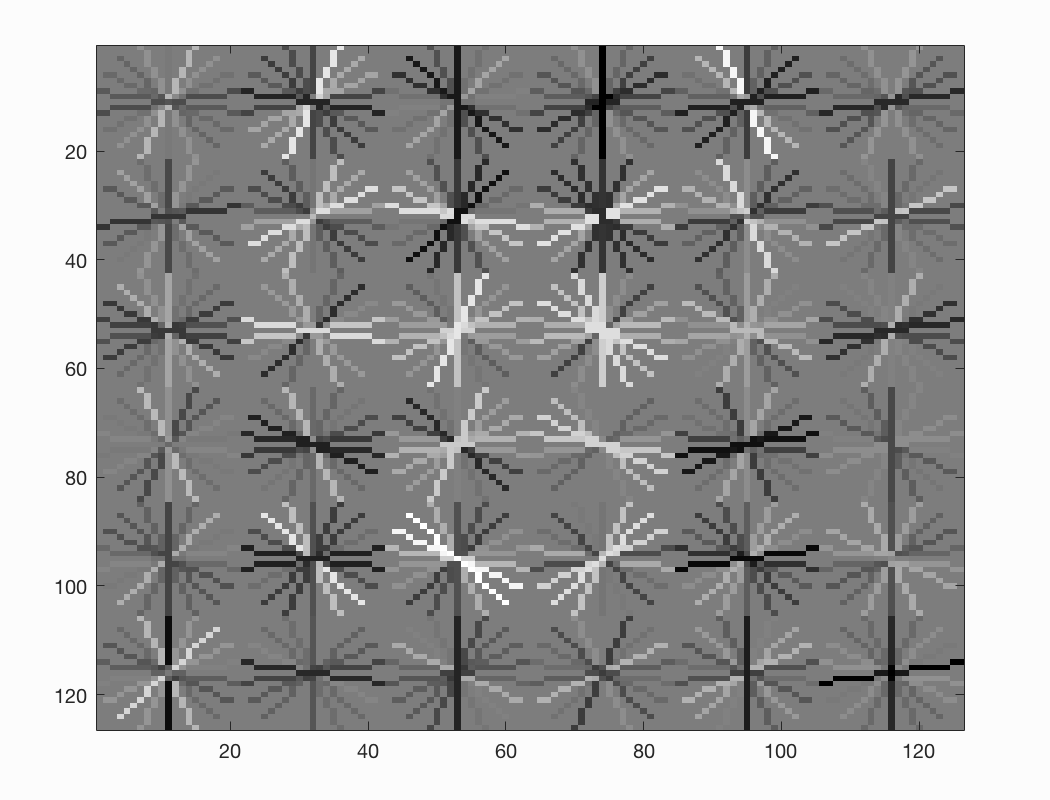
We will use vl_svmtrain on your training features to get a linear classifier specified by w and b. We will implement this in the file proj5.m in the section Step 2. Train Classifier.
- Step 1: We start by creating a lambda variable that will be used in our vl_svmtrain function. We will initially set this to $1x10^{-4}$, and will experiment with this value shortly.
- Step 2: We will create our X variable that will go into vl_svmtrain. To do so we need to create a matrix that has has the first row as features_pos and the secon row as features_neg. To do this we simply do [features_pos; features_neg]. We then take the transpose of this vector so that we do not have dimensionality issues in the vl_svmtrain call.
- Step 3: We get the number of rows in features_pos and features_neg and denote these as s1 and s2.
- Step 4: We create y1 = ones(s1,1) and y2 = -ones(s2,1). Here we take the rows of a vector of ones of size s1 and we take the rows of a vector of negative ones of size s2.
- Step 4: We create a vector Y that has rows y1 and rows y2, Y = [y1;y2].
- Step 5: We compute w and b through vl_svmtrain, [w b] = vl_svmtrain(X,Y,lambda).
Let us now run proj5.m and take a look at the output:
Initial classifier performance on train data:
accuracy: 0.999
true positive rate: 0.404
false positive rate: 0.000
true negative rate: 0.595
false negative rate: 0.001
 Precision/Recall |
 Recall/False Positives |
 P3 |
|---|
We see that our accuracy has increased but our precision is still zero (we will implement the run_detector next and will have an average precision value that is non-zero). Let us implement run_detector.m next and then we can run the full pipeline and parameter tune to see our results.
Run Detector:
This function returns detections on all of the images in a given path. We will use non-maximum suppression on a per image basis on our detections to increase performance. Initially the code returns random bounding boxes in each test image. However, we will change it so that it converts each test image to HoG feature space with a single call to vl_hog for each scale. We will then step over the HoG cells, take groups of cells that are the same size as our learned template, and then classify them. If the classification is above some confidence, we will keep the detection and then pass all the detections for an image to non-maximum suppression.
- Parameters:
- test_scn_path: A string. This directory contains images which may or may not have faces in them.
- w: A parameter in the linear classifier.
- b: A parameter in the linear classifier.
- feature_params: A struct with fields feature_params.template_size (default 36), the number of pixels spanned by each train/test template and feature_params.hog_cell_size (default 6),
- Return Variables:
- bboxes: A vector of size Nx4, where N is the number of detections. bboxes(i,:) is [x_min, y_min, x_max, y_max] for detection i. We note that y is dimension 1 in matlab.
- confidences: A vector of size Nx1. confidences(i) is the real valued confidence of detection i.
- image_ids: A cell array of dimension Nx1. image_ids{i} is the image file name for detection i. This is not the full path.
- Test Scenes: We create a variable called test_scenes where we take the test_scn_path and add '*.jpg' to it. We then use the fullfile and dir function from matlab on
- Empty vectors: We create two vectors and one cell that will be incrementally exapanded throughout our code. bboxes = zeros(0,4), confidences = zeros(0,1), and image_ids = cell(0,1).
- Scale and Setup Variables: After speaking with the teaching assistants it was noted that a scale vector of powers of 0.8 was a good vector to use. Thus, my scale vector was [1,.8,.64,.512,.4096,.32768,.262114,.2097152]. I tried other scale vectors but they lacked in comparison. Additionally, we will be using feature_params.hog_cell_size and feature_params.template_size in our following code a great deal so I created two variables fphcs = feature_params.hog_cell_size and fphts = feature_params.template_size.
- Threshold: We need a threshold to filter our confidences so we set a variable for that. I will set the threshold to 0.7. We will experiment with alternate values in the results section.
- For loop: We iterate over the length(test_scenes) and print the test_scenes(i) name as well as use fullfile and imread on test_scn_path and test_scenes(i).name to get our img variable. We then convert it to a single and divide by 255 so that we have the correct data type and correct values. We then use a conditional to check if the size(img,3) > 1. If it is we turn the image into a grayscale image. If it is not then it is already a grayscale image.
- More Variables: We create some current versions of the variables we created in the setup variables. cur_bbox = zeros(0,4), cur_confidences = zeros(0,1), and cur_image_ids = cell(0,1).
- Nested for loop: We iterate over length(scale). We then let scale_val be the scale(j) and resize our image by the scale_val, we denote this as variable scaled_img. We then get the height (hgt) and width (wdth) of scaled_img. We use vl_hog(scaled_img, fphcs) and store this in the test_f variable. This variable will hold our test features. We now construct a window variable and get the x as floor(wdth/fphcs) - (fphts / fphcs) + 1 and the y as floor(hgt/fphcs) - (fphts / fphcs) + 1. We need a dimension which will be 31*((fphts / fphcs)*(fphts / fphcs)). Our window will then be zeros((floor(wdth/fphcs) - (fphts / fphcs) + 1)(floor(hgt/fphcs) - (fphts / fphcs) + 1),31*((fphts / fphcs)*(fphts / fphcs))).
- Double for loop: We iterate k over x_window and l over y_window where x_window = floor(wdth/fphcs) - (fphts / fphcs) + 1 and y_window = floor(hgt/fphcs) - (fphts / fphcs) + 1. We use the floor function just in case we do not get a whole number if we change parameters in the proj5.m file. We then let our index be indx = (k-1)*y_window+l and we add test_feat = reshape(test_f(l:(l+ (fphts / fphcs) - 1), k: (k+ (fphts / fphcs) - 1),1,31*((fphts / fphcs)*(fphts / fphcs)))) into window(indx,:).
- Next Steps:We then calculate src = (window*w)+b and find the indices of scr that are greater than the threshold. We then let scl_conf be scr(these indices). We then calcualte our_x = floor(ind./y_window) and our_y = mod(ind,y_window)-1.We then calculate scl_bboxes = [scl_bbox_one, scl_bbox_two, scl_bbox_three, scl_bbox_four] where scl_bbox_one = fphcs*our_x+1, scl_bbox_two = fphcs*our_y+1, scl_bbox_three = fphcs*(our_x+(fphts / fphcs)), and scl_bbox_four = fphcs*(our_y+(fphts/fphcs)). We then take scl_bbox and perform element-wise division with our scale_val. Now we create scl_img_id = repmat({test_scenes(i).name}, size(ind,1), 1). Finally we calculate our cur_bbox, cur_confidences, and cur_image_ids where cur_bbox = [cur_bbox; scl_bboxes], cur_confidences = [cur_confidences;scl_conf], and cur_image_ids = [cur_image_ids; scl_img_id].
- Non-Maximum Suppression: We perform non-maximum suppression to get the is_maximum and then take the maximum of cur_confidences, cur_bbox, and cur_image_ids.
- Return Variables: We then create bboxes = [bboxes;cur_bbox], confidences = [confidences;cur_confidences], and image_ids=[image_ids;cur_image_ids]. We then return bboxes, confidences, and image_ids.
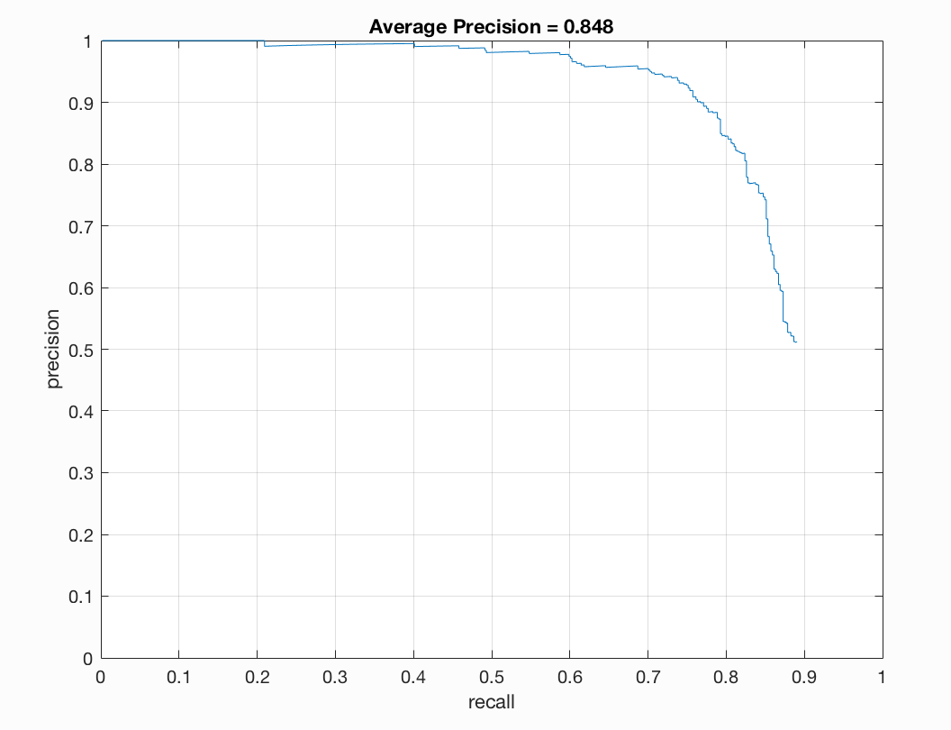
With these steps we should now get a precision that is not zero. Let us run our pipeline with a different set of thresholds, lambdas, scales, and sample sizes and examine the average precision:
| Threshold | Lambda | Scale | Num Samples | Average Precision |
|---|---|---|---|---|
| 0.7 | 0.0001 | 6 | 10,000 | 0.841 |
| 0.6 | 0.0001 | 6 | 20,000 | 0.832 |
| 0.8 | 0.0001 | 6 | 10,000 | 0.818 |
| 0.7 | 0.0001 | 6 | 11,500 | 0.813 |
| 0.4 | 0.0001 | 6 | 15,000 | 0.841 |
| 0.67 | 0.0001 | 6 | 15,000 | 0.803 |
| 0.7 | 0.001 | 6 | 12,000 | 0.835 |
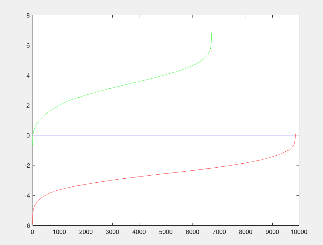
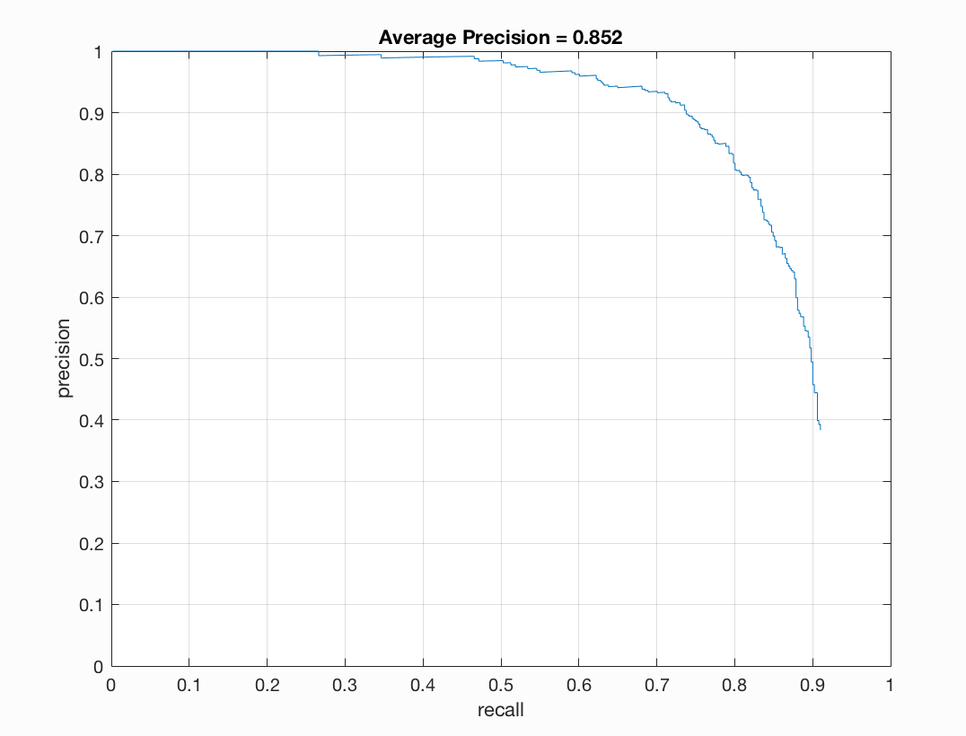
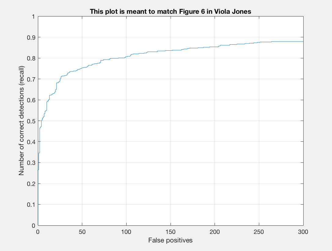
| 0.7 | 0.0005 | 6 | 12,000 | 0.852 |
I found that a lambda of 0.0005 worked best for me. This regularization parameter is important for training our linear SVM. If it is too high or too low we will get underfitting or overfitting on our training data. A threshold of 0.7 worked nicely for me. Here there was a good balance between accuracy and minimization of red boxes on our images. If I lower the threshold too much than there is better precision but more red when we examine the test output. I noticed that the number of samples did not make a drastic difference for me. When bumping up from 10,000 to 11,000 or 12,000 there was a slight positive difference. With 20,000 I did not notice too much of a difference that was justifiable with the addional computational expense incured. To get the best precision I used a lambda of 0.0005, a threshold of 0.7, and 12,000 as num_negative_examples.
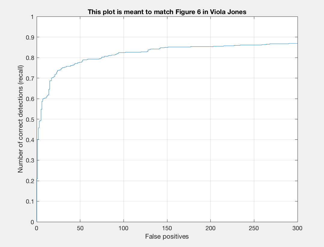
Some output for this set of parameters is as follows:
 Precision/Recall |
 Recall/False Positives |
 P3 |
 P4 |
|---|
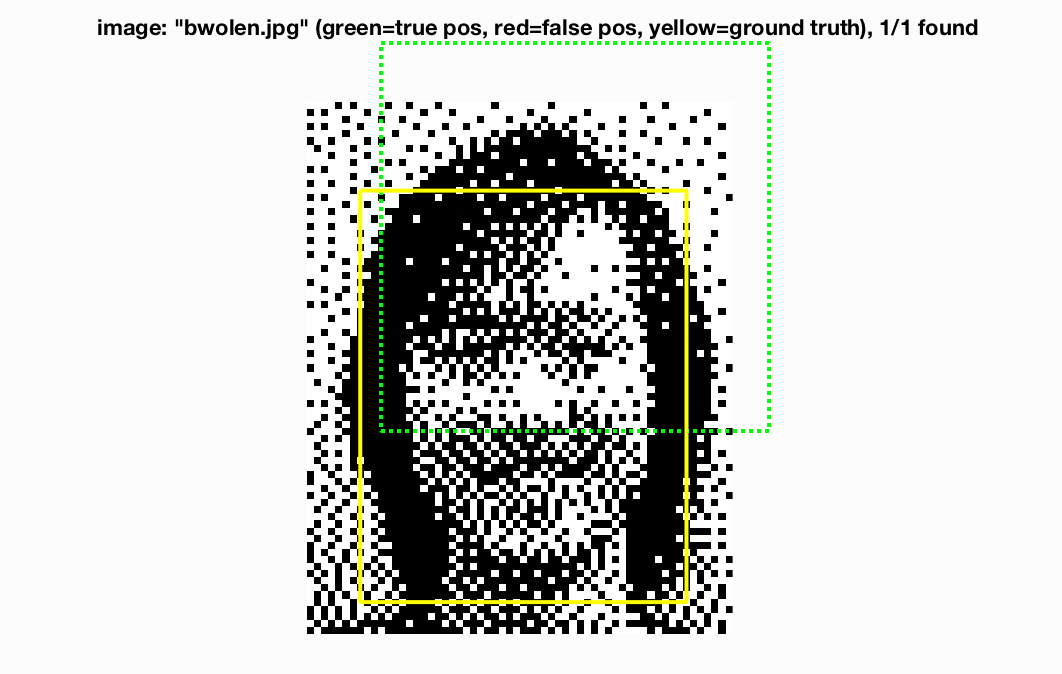
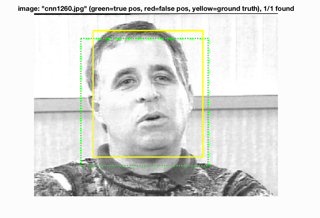
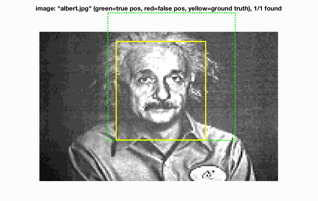
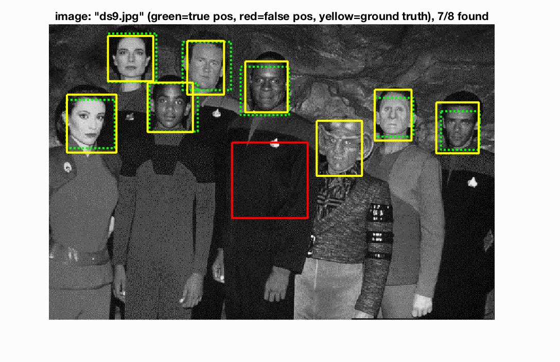
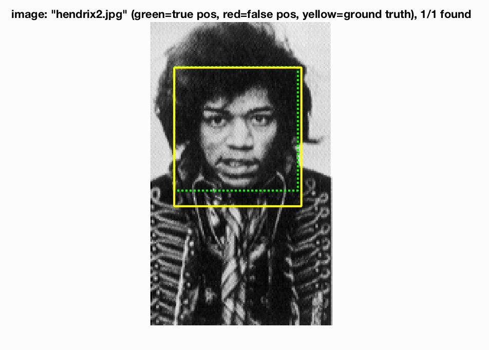
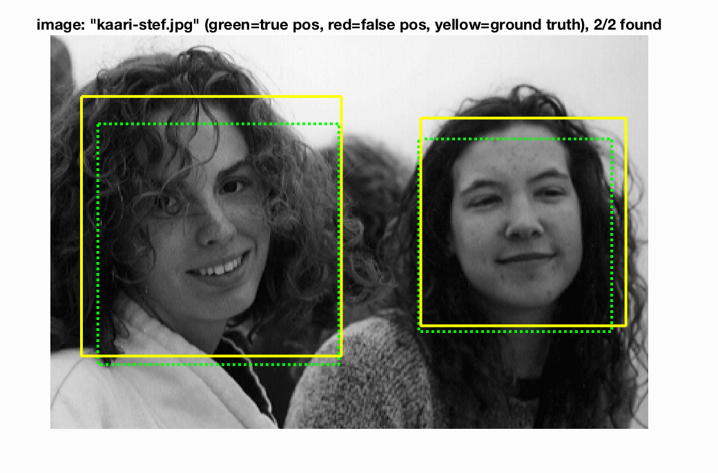
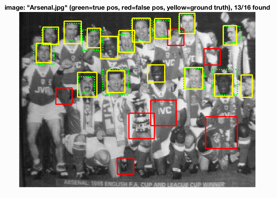
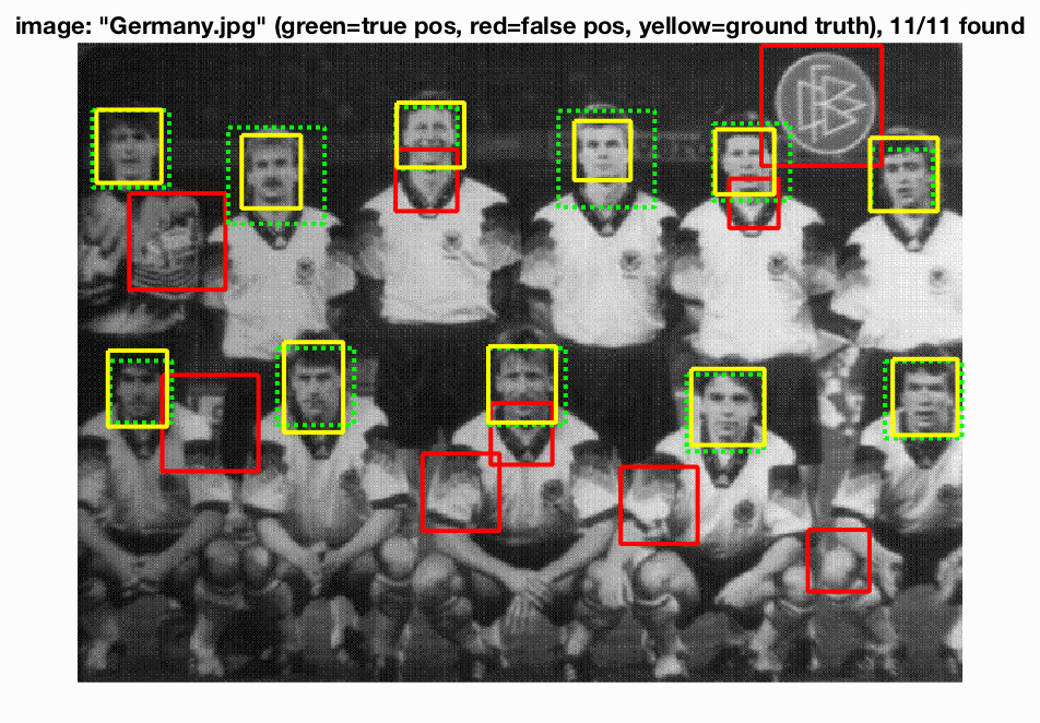
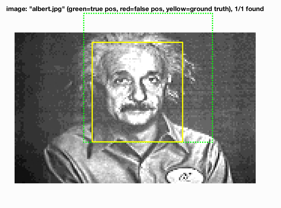
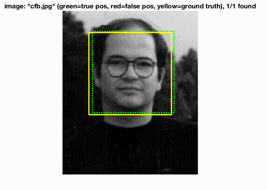
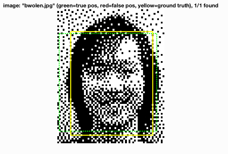
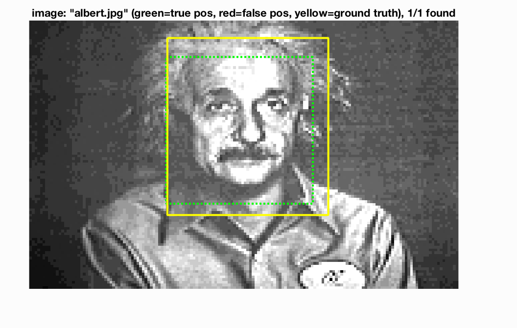
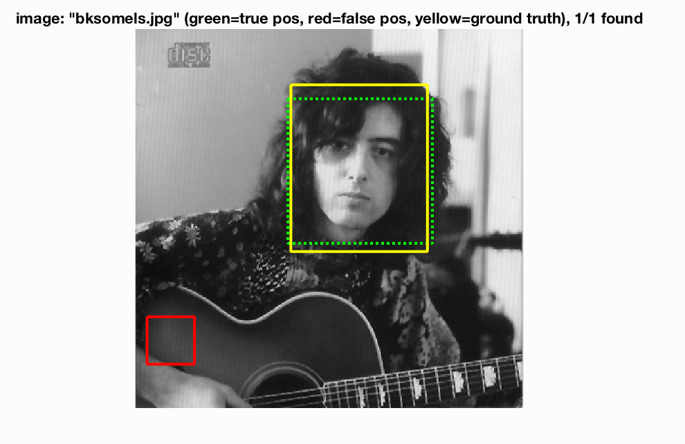
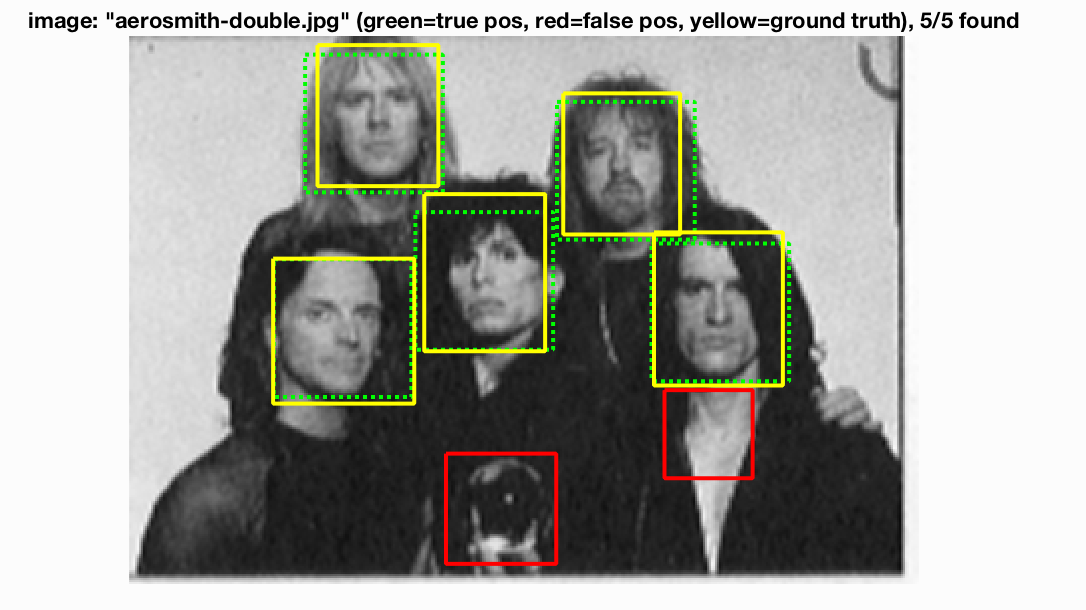
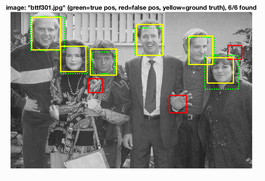
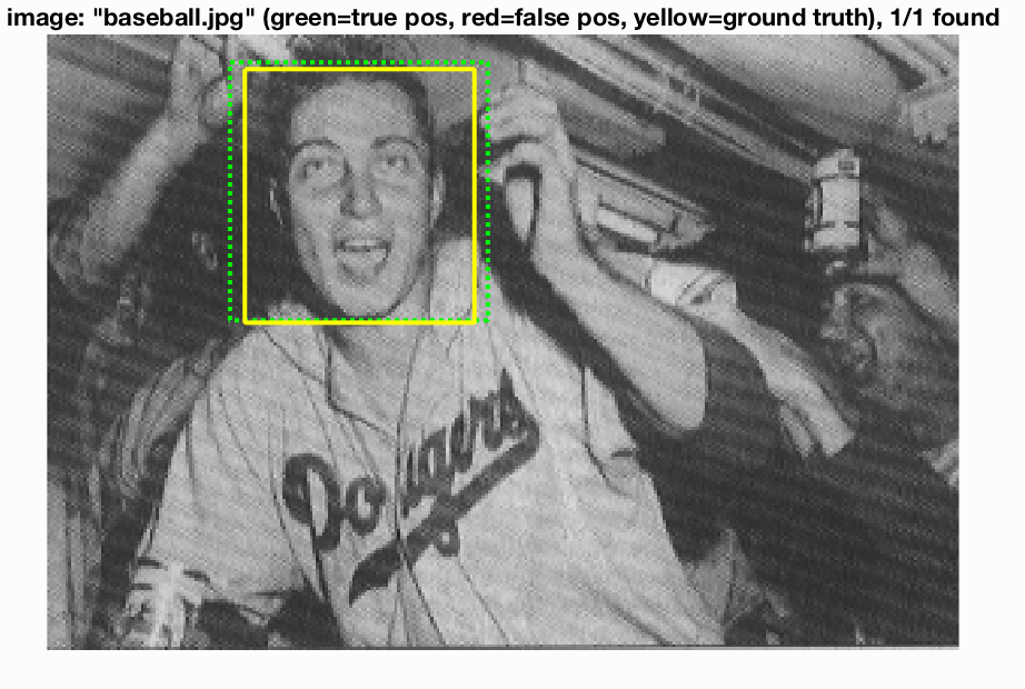
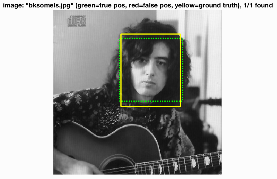
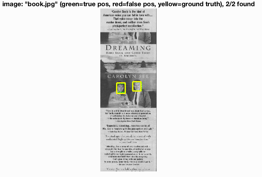
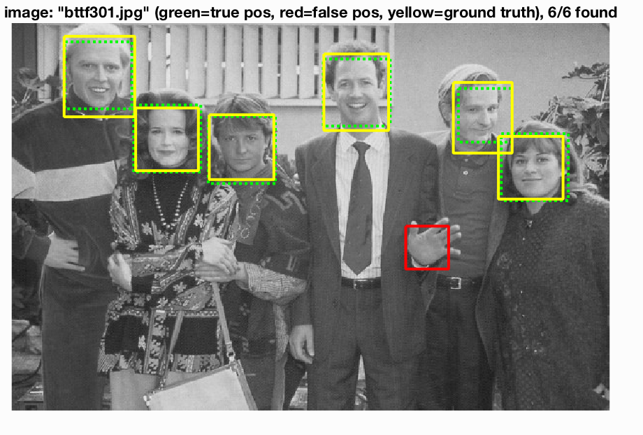
Some test output is as follows:
 |
 |
 |
 |
|---|---|---|---|
 |
 |
 |
 |
 |
 |
 |
 |
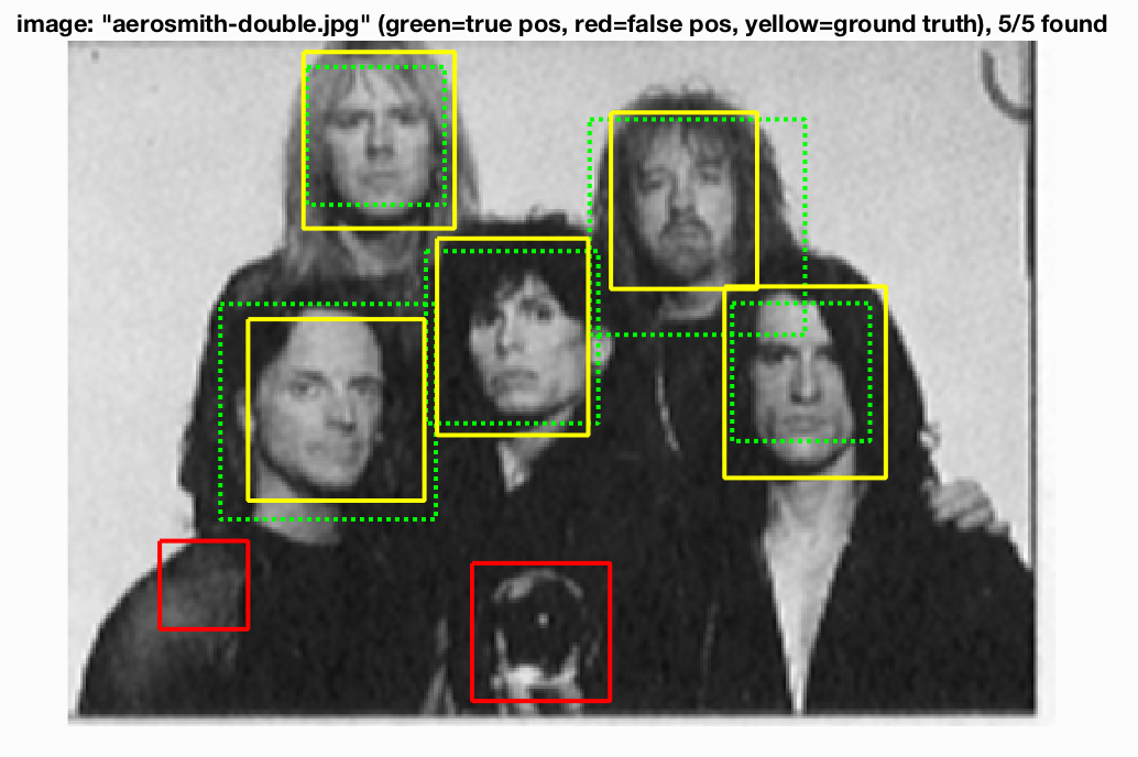
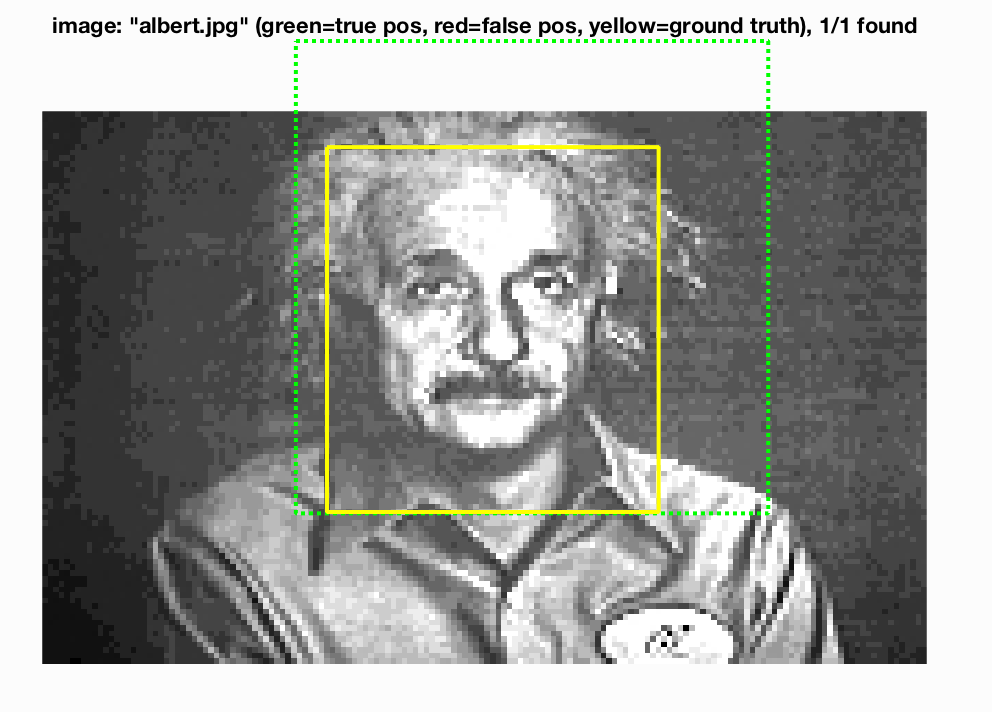
We see that for the most part our face recognition came out pretty nicely. There are some false positives in the bottom images but we are finding faces a good percentage of the time.
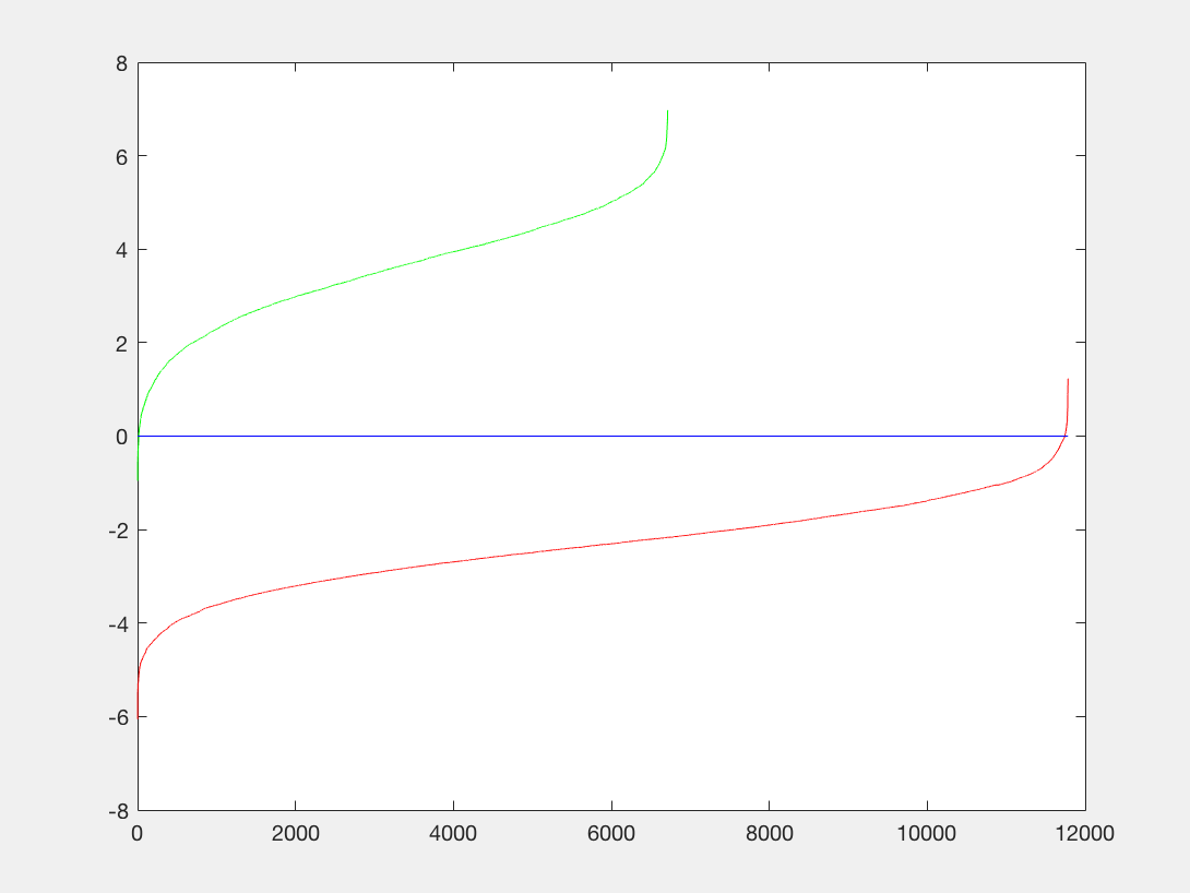
Let us take a look at another setup of parameters for comparison: lambda = 0.0001, threhsold of 0.7, and 15,000 negative samples:
 |
 |
 |
 |
|---|
Some test output is as follows:
 |
 |
 |
 |
|---|---|---|---|
 |
 |
 |
 |
 |
 |
 |
 |
We see that the lambda of 0.0005 did better for our program. We had more face findings and had less false positives. If we were to lower our threshold more we would see much more false positives but most likely higher precision.
Let us now use our parameters lambda = 0.0005, threshold = 0.7, and num_negative_samples = 12,000 and examine the average precision with different pixel cell sizes:
| Threshold | Lambda | Scale | Num Samples | Average Precision |
|---|---|---|---|---|
| 0.7 | 0.0005 | 6 | 12,000 | 0.852 |
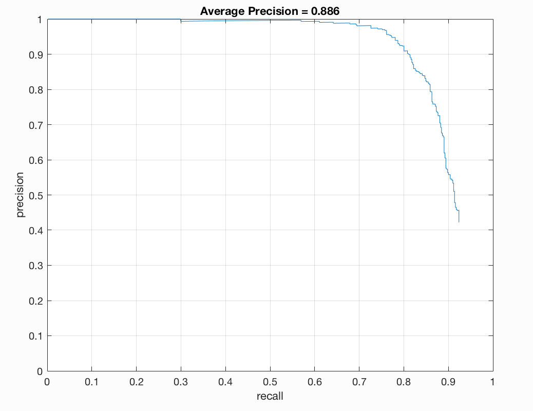
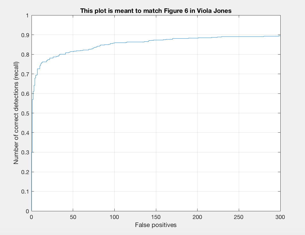
| 0.7 | 0.0005 | 4 | 12,000 | 0.886 |
| 0.7 | 0.0005 | 3 | 12,000 | 0.918 |
With a 4 pixel cell size our results were as follows:
 |
 |
 |
 |
|---|
Some test output is as follows:
 |
 |
 |
 |
|---|---|---|---|
 |
 |
 |
 |
Some output images for the 3 pixel cell size are as follows:
 |
 |
 |
 |
|---|---|---|---|
 |
 |
 |
 |
We note that the 3 pixel cell size with our combination of parameters gives us the best precision and facial matching, however it is computationally expensive. The best combination of precision and speed was a 4 pixel cell size, which took roughly 6 minutes and 45 seconds to run, producing an average precision of approximately 0.873 across 10 runs of the program.
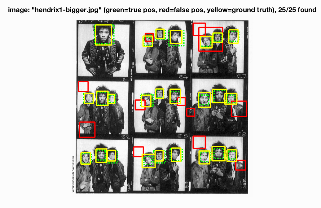
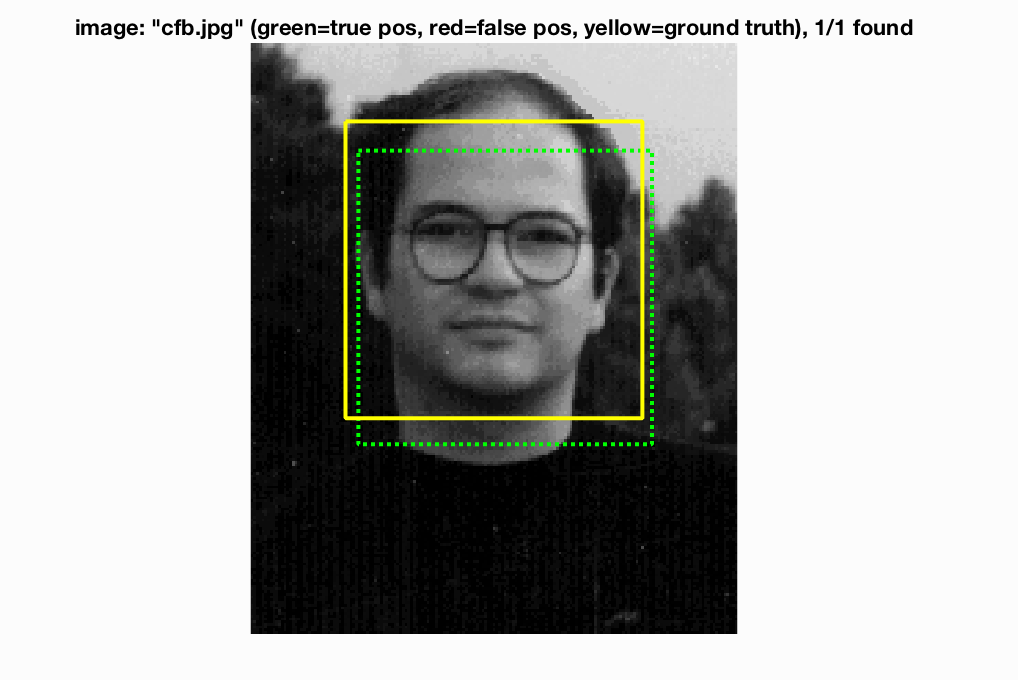
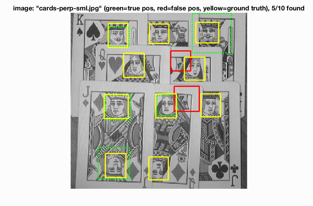
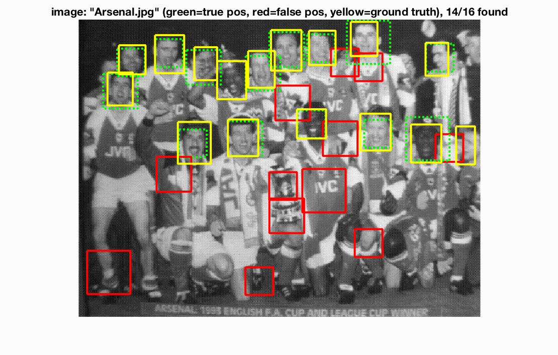
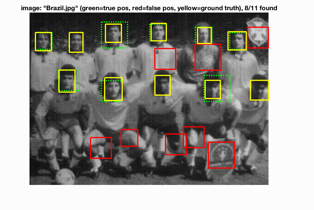
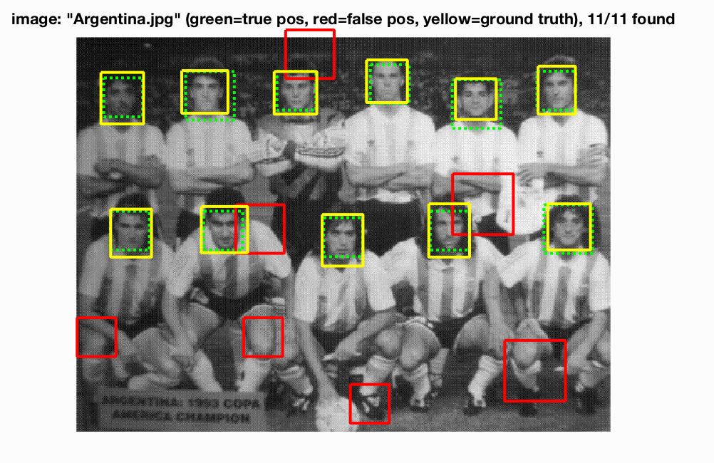
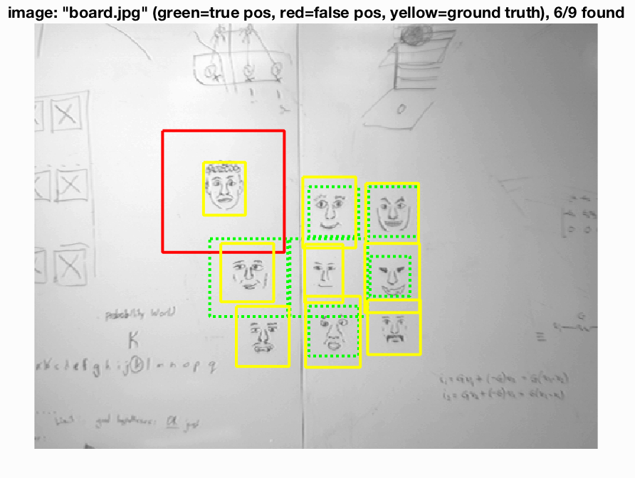
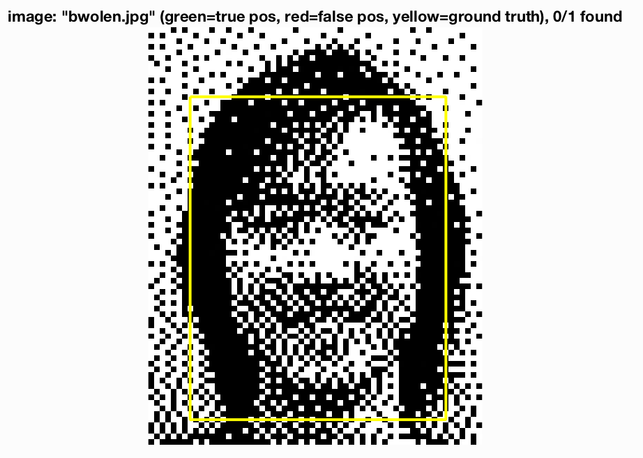
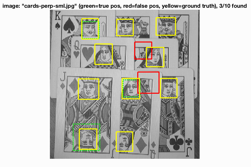
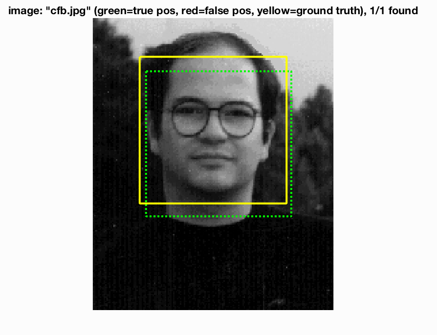
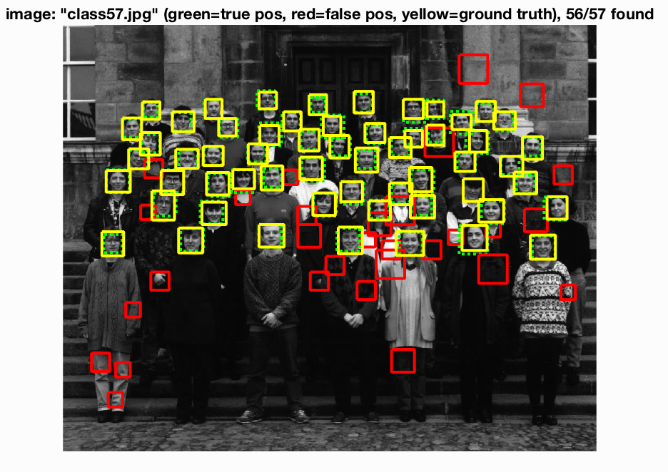
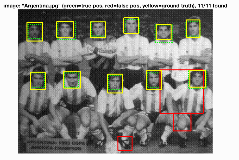
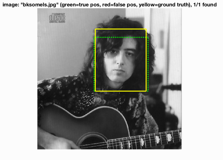
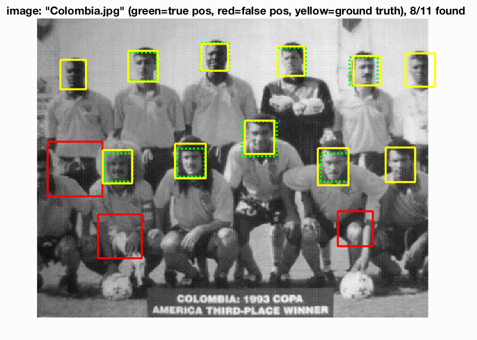
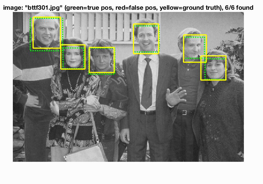
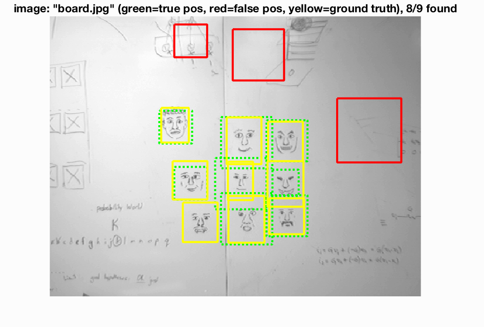
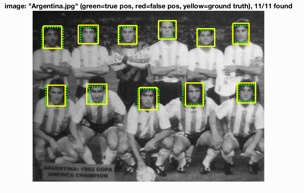
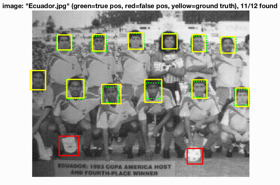
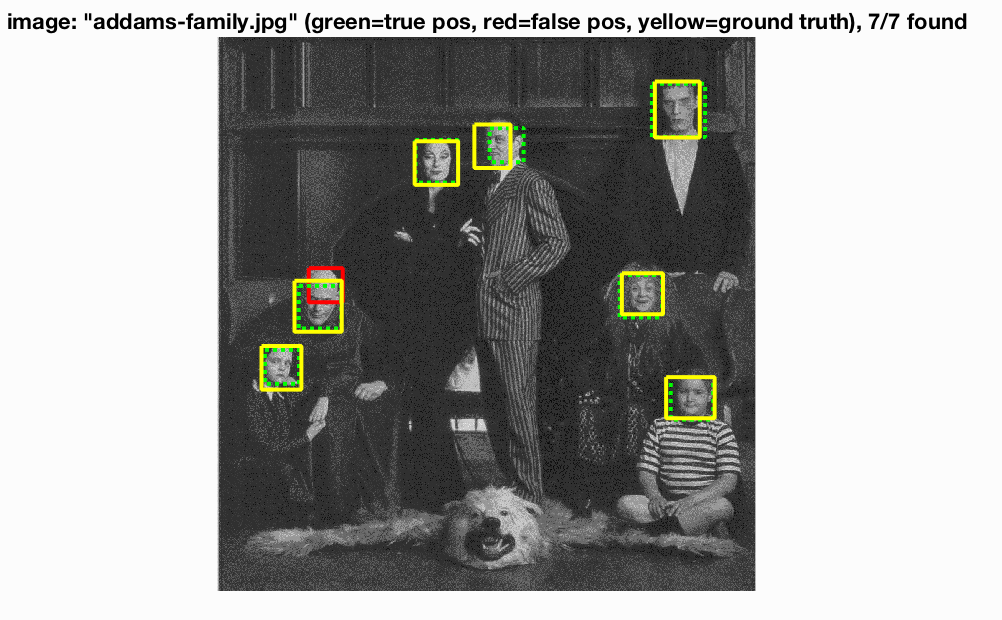
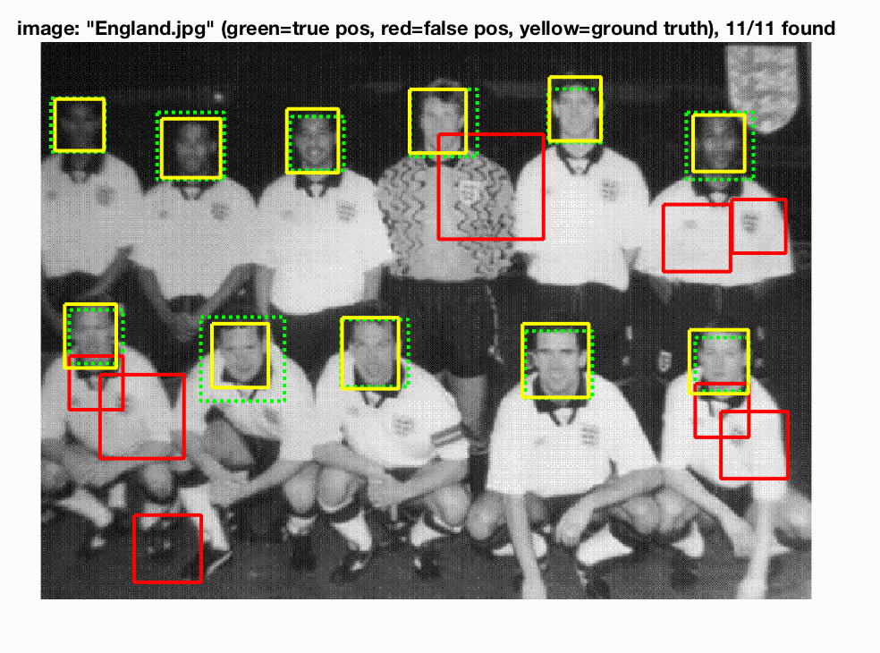
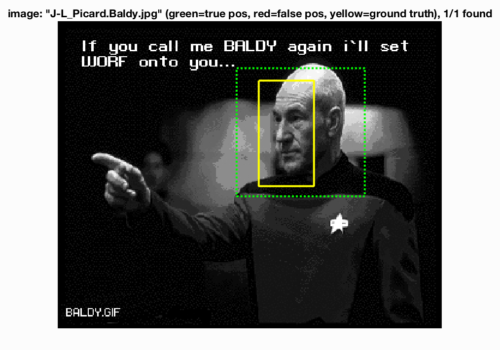
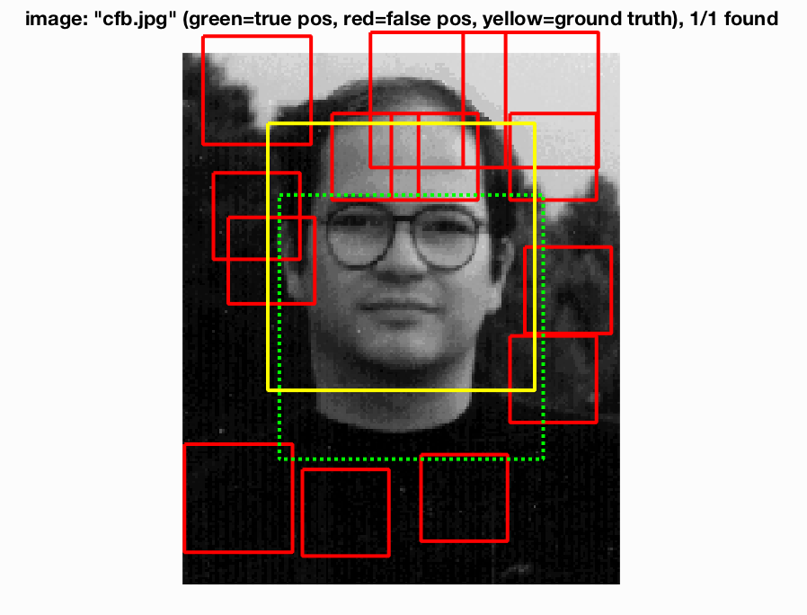
Let us now run our code with the class test images. The results are as follows:

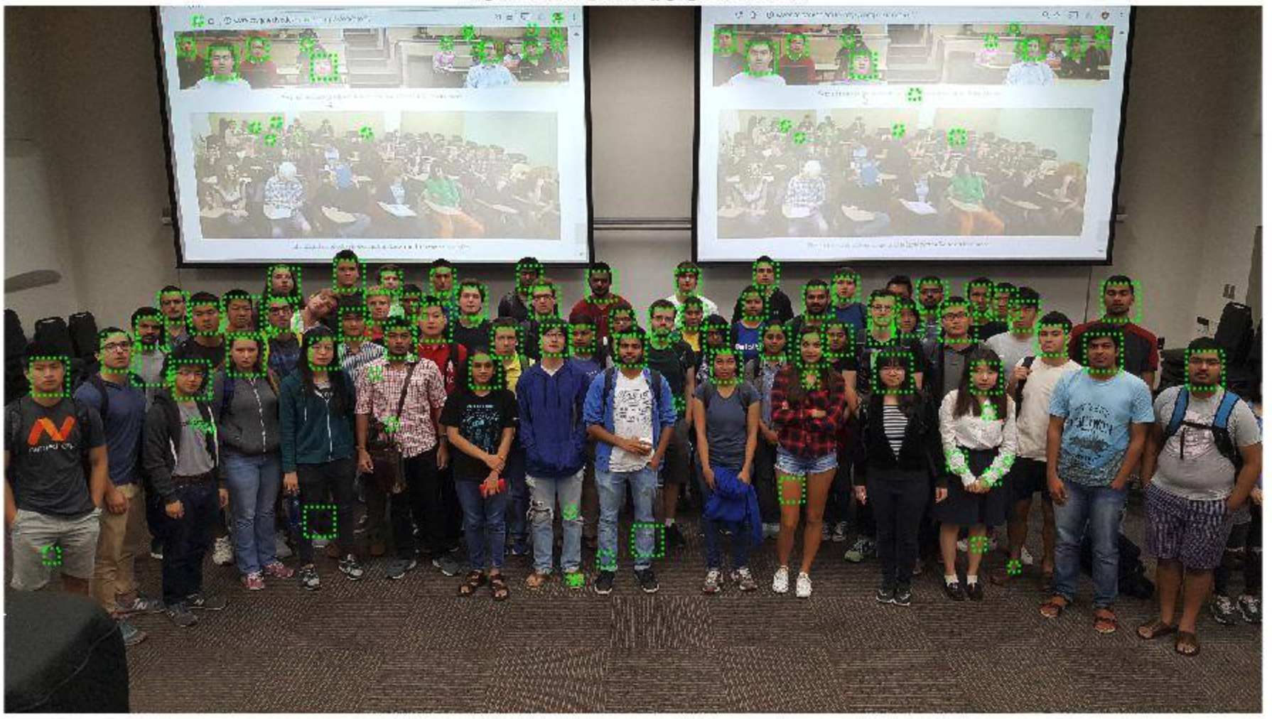
We see that for the most part, the face detection is pretty good despite the few incorrect green boxes we have. Note: I had memory issues with my machine and had to do some rescaling of the images to get the vectors to not exceed memory allocations.
Graduate Extra Credit:
We will be implementing hard negative mining for our graduate extra credit. Let us quickly summarize what hard negative mining will do for us. Say I give you a collection of images and bounding boxes for each image. Our classifier will need both positive training examples (face) and negative training examples (non-faces). Our positive training examples come from looking inside the bounding box for each person/image. However, how do we create useful negative training examples? If we generate a bunch of random bounding boxes and for each that does not overlap with any positives, we keep that as a negative. We now have some positives and negatives, so we can train a classifier and test it with our training images and a sliding window. However, this may give us a high amount of false positive. It might be thinking that there are faces when there are not. We can use a hard negative to falsely detect a patch, and explicitly create a negative example from that patch. We can then add that negative to our training set. Now upon retraining the classifier we should have better performance as we have additional knowledge. Now, we should have less false positives.
Our implementation is as follows:
- New run_detector.m: We first create a new run_detector called run_detector2.m. The reason for this is that we want to have a different threshold than the run_detector that we will call later. In run_detector2, I also specify a parameter that will allow me to make non-maximum suppression a conditional as it might be a hinder to our negative hard mining. With this, we can copy our code over from the original run_detector and make the changes above. This time we will take in non_face_scn_path, w, b, feature_params, and 1 or 0. Where 1 means we use non-maximum suppression and 1 means we do not skip non-maximum suppression. We will then output hard_m_bbpoxes, hard_m_confidences, and hard_m_image_ids
- Confidences Threshold: We will let t be our new threshold to filter our confidences after we run run_detector2.m.
- Filter Confidences: We use matlab's find function to see where the hard_m_confidences are greater than the specified threshold. We store this in a variable called hard_m_indx
- Setup Variables: We let l be the number of columns in hard_m_bboxes and we create two empty vectors: vec and c. These vectors will have incrementally added elements in the for loop which we will describe next.
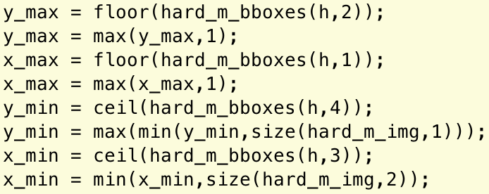
- For loop: We iterate over l and strcat our non_face_scn_path with '/' and hard_m_image_ids{h} where h ranges from 1 to l. We then read it in, turn it to gray if it is not already a grayscale image, and then cast it to a single data type. We then need to calculate y_max, x_max, y_min, and x_min, where we call the function get_maxes(hard_m_img,hard_m_bboxes,h) to get [y_max, x_max, y_min, x_min]. The computation inside this function is seen below.
- Get new w and b: We create a function called get_new_w_b which takes in a classifier_lambda, features_pos, features_neg, and c. It uses vl_svmtrain on a feature we create from feature_pos, feature_neg, and c and the classifier lambda value, which we set to 0.0005. We then return new_w and new_b.
- run_detector: We finally call [bboxes, confidences, image_ids] = run_detector(test_scn_path, new_w, new_b, feature_params).
Let us now parameter tune and see which values work best for our hard_mining.m function:
With a t=0.85, a threshold of 0.8 in run_detector2, a classifier_lambda = .0005, and a 6 pixel cell size our results are the following:
 |
 |
 |
 |
|---|
Some test output is as follows:
 |
 |
 |
 |
|---|
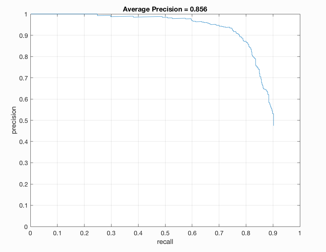
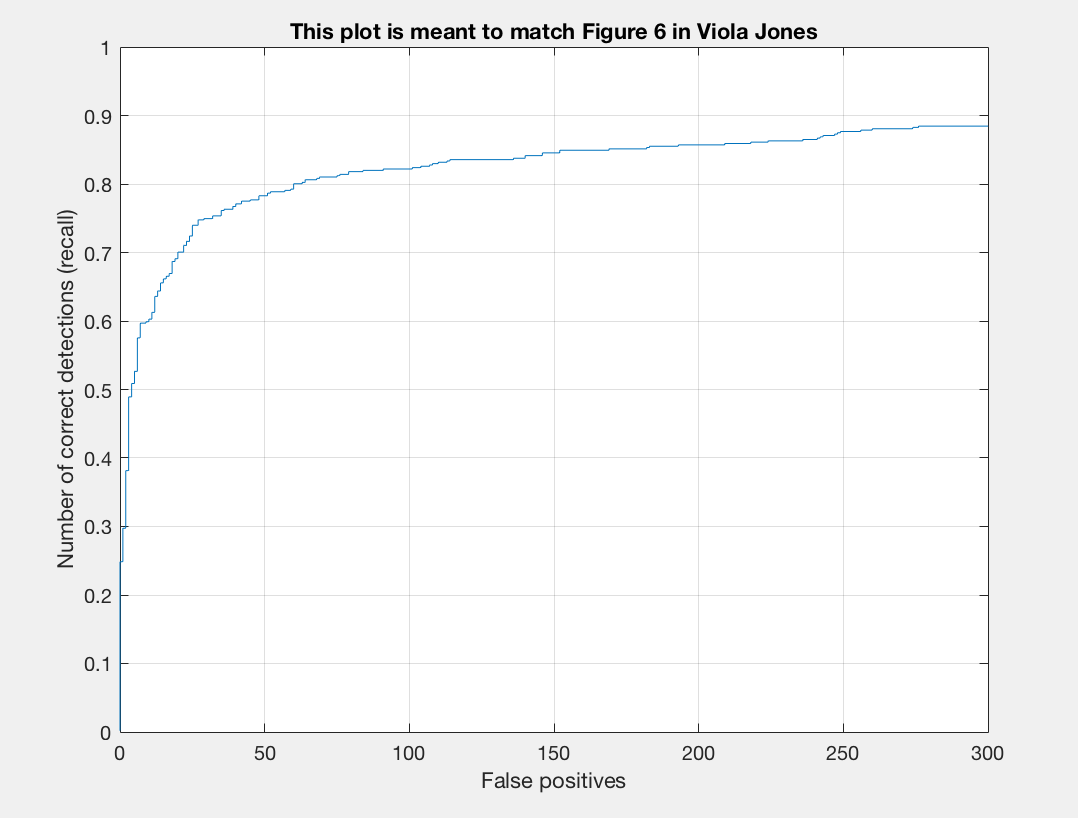
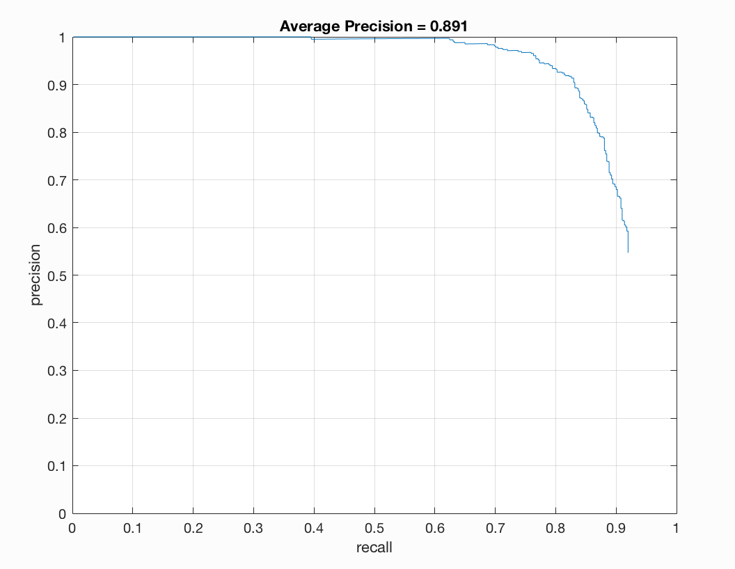
Previously, we were getting around 81-83% but now we are getting over 85% precision. After turning parameters, with a cell size of 6, I ultimately arrived at a precision of 89% on one run of my program. The plot is as follows:
When we use a cell size of 4, our precision is slightly larger than that of what we previously had. However, there is not as much of a difference as there is in the 6 pixel cell size.
Thus, we see that using the negative hard mining has helped! In terms of computational complexity, it does not cost too much and gives us slightly better results so it is definitely a worthwile implementation.
Here, we are going to augment our data and see how the precision changes.
To track all our changes we will implement a new file: augmented.m that will depend on augmented_pos_feats.m and augmented_neg_feats.m. These two files are copies of our get_positive_features and get_random_negative_features except they have some code that alters the training data.
Let us first flip the rows in our image horizontally. This will flip our image. We can make use of matlab's built-in function flipud for this. After flipping our training data and using the same parameters as above with a 6 pixel cell size we see that our output is as follows:
 |
 |
 |
 |
|---|
Compared to our previous output of ~83%, we see that our precision has dropped a great deal but we are still getting around 50% precision! This is very interesting as it seems like we are still detecting faces even with upside down faces as our training data.
Looking through some of the training examples, I noticed that some of them were slightly blurry. Let us now sharpen our image and see if we get any improvement in accuracy.
 |
 |
 |
 |
|---|
We see that our accuracy went up a slight bit. I re-ran the program and constantly achieved a slightly higher precision with the sharpening. This seems to help a few of the blurry images become more easily recognizable for face detection.
Let us try filtering our image with a gaussian filter, so we have a blurred effect. My hypothesis is that the precision will drop as the images are harder to detect so our classifier will have a hard time. Let us check out the results below:
 |
 |
 |
 |
|---|
The precision dropped significantly! We are now down from low-mid 80% to high 60-low 70%. Blurring our image really did make a difference in terms of facial recognition.
Now, let's really enahnce the colors of our images using matlab's decorrstretch and imcoloradjust. We will use a coloradjust of ([.10,.79],[0.00,1.00],1.10). Here the image will look more vibrant. The results are as follows:
 |
 |
 |
 |
|---|
We see that our precision here is on par with our original test data.
Let us now overlay the a cropped version of the image over itself and turn it a slight green/yellow color. We will rotate the original image using 5,'bicubic','crop' and then we will fuse this rotated and transformed image with the original image and use the parameters 'falsecolor','Scaling','joint','ColorChannels',[1 2 0]. This might cause some confusion to the image, it will make it look like its been all shaken up. Let's take a look at the precision plots below:
 |
 |
 |
 |
|---|
Our precision here is terrible we have dropped into the 50's from the 80's. The shaken double effect really made it difficult to detect a face here.
Let us run a Canny Edge detection on each image and use this array as our training data. I have some worries here as we do not have pictures with bland backgrounds of just a face. We have scenery in our image so I am predicting that our classifier is going to perform very poorly here. If there are buildings and other scenery, I forsee this trying to detect these as faces. The results are as follows:
 |
 |
 |
 |
|---|
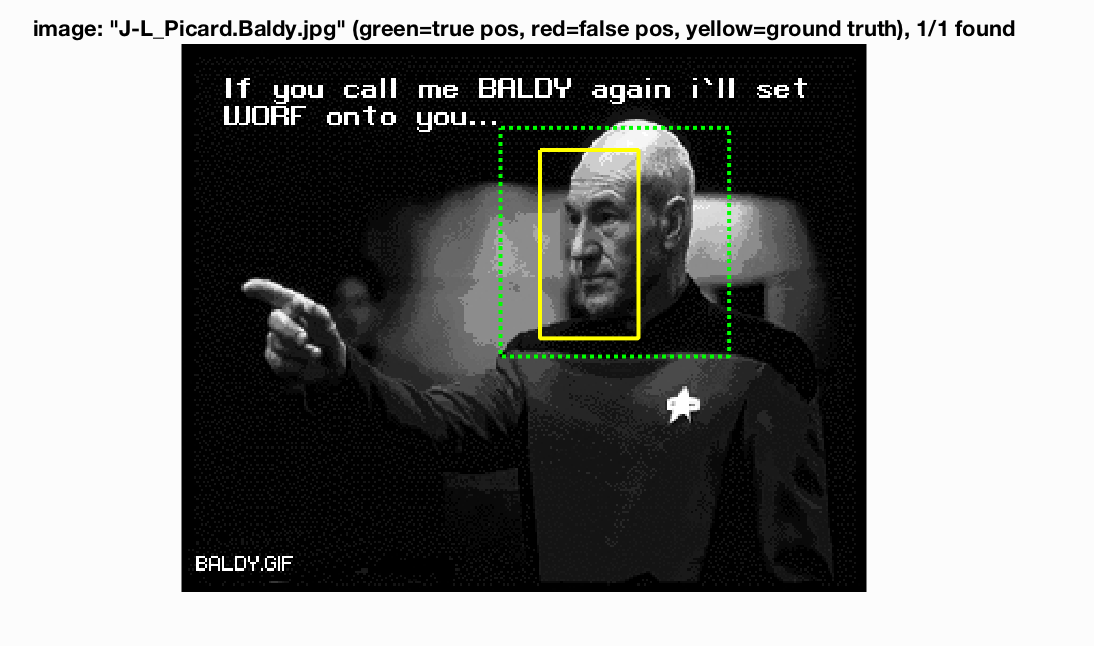
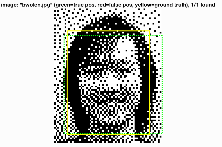
As we can see, this did in fact do very poorly. If we take a look at one of the produced output's below
we see that the bounding boxes were looking at the edges that defined the man in the figure. Using the canny image detector might be better for classifying some other object that is not a face, such as a particular car model for instance.
All in all we see that augmenting and filtering our training data did have an effect on the final average precision. When we sharpened our image we got slighly higher average precision. When we blurred our training data we had lower average precision. When we applied some strange filters to our training data we also had lower average precision especially when we used the canny edge detector. So, augmenting our training data did make a substantial impact. There is no huge computational expense associated with augmenting the data as my program only took a few more seconds to run, but sharpening the images was a nice small bump in average precision. The files used in the above implementations are augment.m, augmented_pos_feats.m, and augmented_neg_feats.m. To run the program you simply go into augmented_pos_feats and augmented_neg_feats and select the augmentation you want on the training data. You then run augmented.m.
Conclusion:
We saw that as we implemented the pipeline we saw an increase in the average precision. There was a good bit of parameter tuning, but after finding the right parameters the average precision was very nice. For extra credit I implemented Hard Negative Mining where I saw a nice boost in average precision and noticed that there were much less false positives. In addition, I implemented new training data through augmentation. I looked at a variety of shapes of the data and combinations of filters of the data to see how the average precision changed as a result of this change in data. I noticed that for some combinations such as sharpening the average precision increased, but for some combinations such as a more color intense cropped verison of the image overlayed with itself the average precision dropped sharply. This makes it easy to undestand that our training data is important. If we have poor quality or confusing training data, then our resulting test data precision will not be as strong as we would hope for. I had a great time implementing this project. I have always been interested in facial recognition and I was finally able to implement my own facial recognition program! This was a great project!
Sources:
- Dr. James Hays' powerpoint slides
- http://www.pyimagesearch.com/2015/03/23/sliding-windows-for-object-detection-with-python-and-opencv/
- http://www.cc.gatech.edu/~hays/compvision/proj5/papers/dalal_triggs_cvpr_2005.pdf
- https://www.quora.com/What-is-Precision-Recall-PR-curve
- http://tinyurl.com/hard-mining-negative
- http://blogs.mathworks.com/steve/2012/11/27/image-effects-part-3/