Algorithm Description

get_positive_features.m

We basically extract all HOG features from each image of the positive training set and append all the projects together.

get_random_negative_features.m

We extract HOG features from the negative image set, randomly choosing approximately num_samples number of negative samples for the negative feature set.

classifier training

We append the positive and negative features and their corresponding labels to form the training data. We then train an SVM to obtain weight vector and offset. This is implemented in proj5.m

run_detector.m

We take each individual image and convert it into HOG feature space. Then we run sliding window on the HOG space and calculate the score of each HOG feature using the trained SVM weights and offsets. We then thresholdthe score and find the bounding boxes in the original image using the coordinates of this HOG block(in the sliding window). We perform non maximum suppression on the bounding boxes. This is performed at various scales of the test image.

Extra Credit

Hard Negative Mining: Ran the trained SVM on the negative train images and used the false positives generated as negative samples for actual run. Result is reported below.

Alternative Positive Training Data: Used mirrored faces from the training data. Also used rotated training images to get more positive features. Used rotation of +10 and -10 degrees.

Example of code with highlighting

%example code- get_positive_features.m 
IM=single(imread(strcat(char(train_path_pos),'\',image_files(i).name)));
HOG = vl_hog(IM, feature_params.hog_cell_size);
features_pos(k,:)=reshape(HOG,[1,D]);

%example code- get_random_negative_features.m
i_min=randi(i_range-g+1,1,1);
j_min=randi(j_range-g+1,1,1);
curr_block=HOG(i_min:i_min+g-1,j_min:j_min+g-1,:);
features_neg(n,:)=reshape(curr_block,[1,D]);

%example code- classifier training
Y=cat(1,Y_pos,Y_neg);
X=cat(1,features_pos,features_neg);
[w, b] = vl_svmtrain(X', Y', lambda);

%example code- run_detector.m 
y_min=r*cellsize/scale;
y_max=y_min+(35/scale);
x_min=c*cellsize/scale;
x_max=x_min+(35/scale);
cur_bboxes=[cur_bboxes;[x_min, y_min, x_max, y_max]];
cur_image_ids=[cur_image_ids;{test_scenes(i).name}];

RESULTS

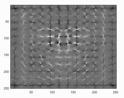
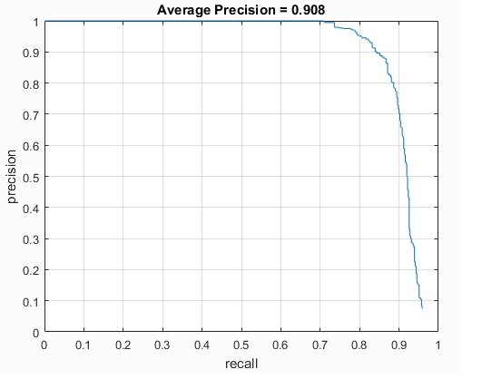
Highest accuracy obtained for cell size 3 is 90.6.

Number of scales of test image =10

Threshold =-0.5

Face template HoG visualization

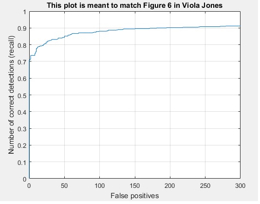
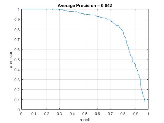
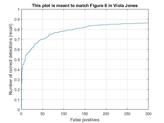
Best Precision Recall curve

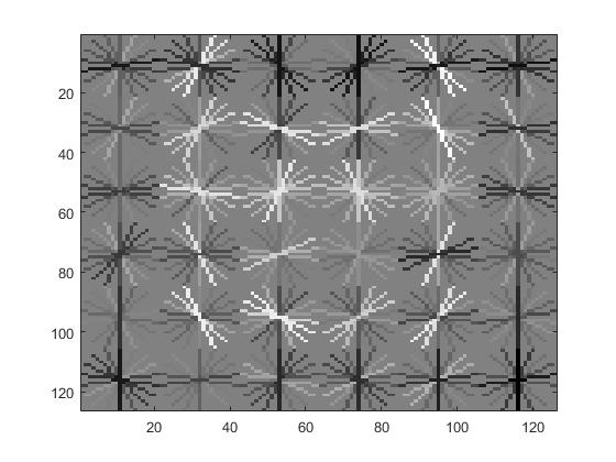
Highest accuracy obtained for cell size 6 is 84.2.

Number of scales of test image =10

Threshold =-1

Face template HoG visualization

Best Precision Recall curve

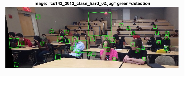
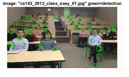
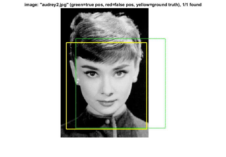
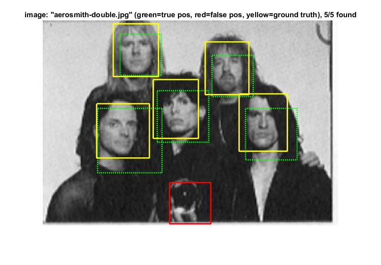
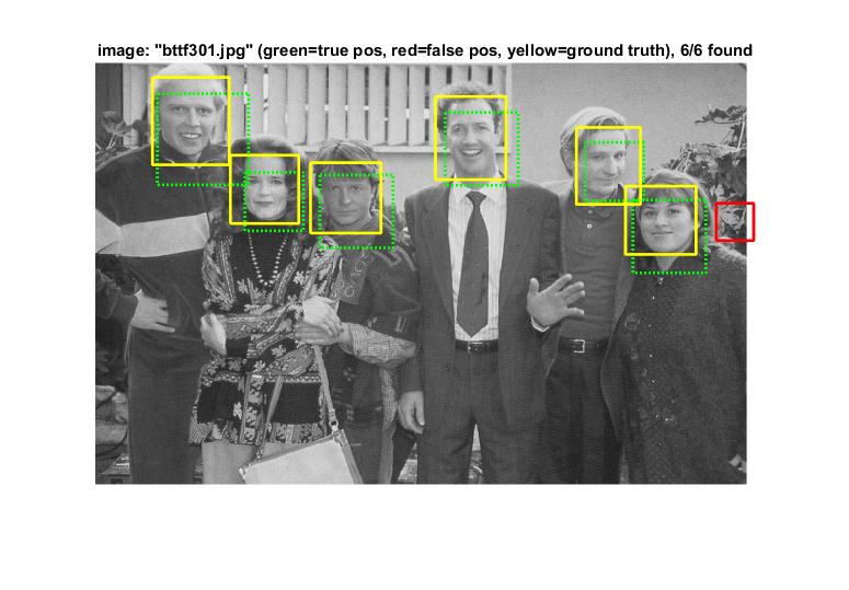
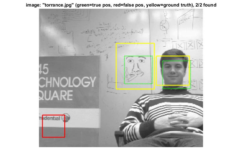
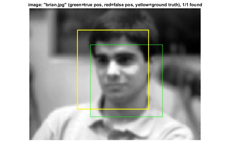
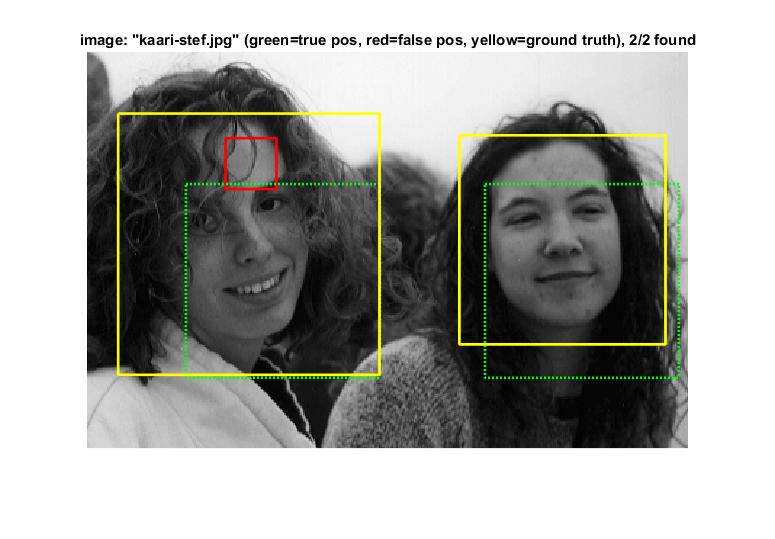
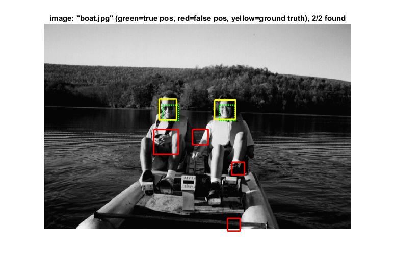
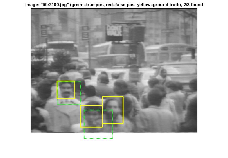
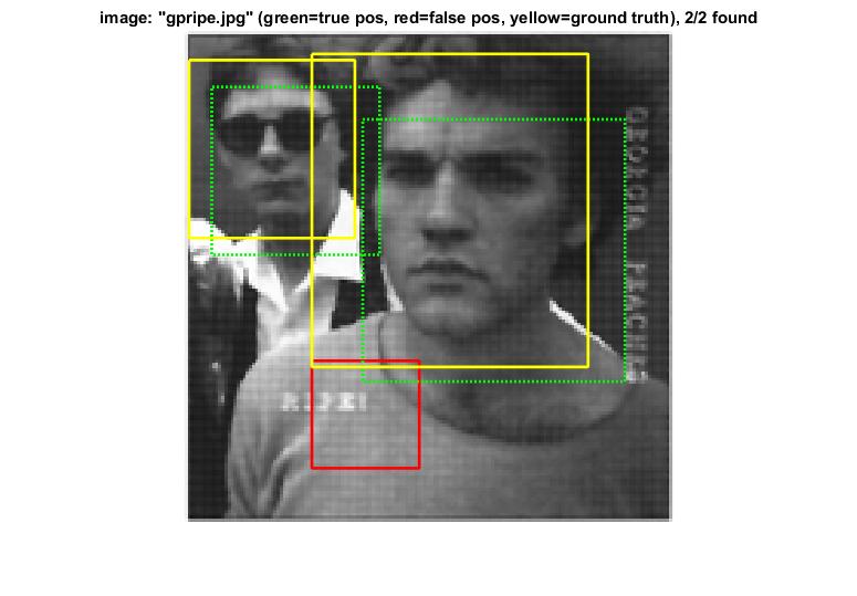
Example of detection on the test set(high threshold)

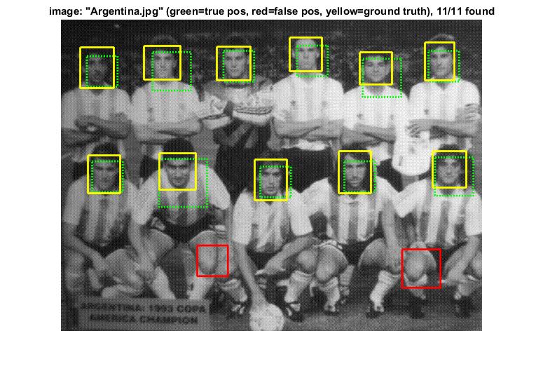
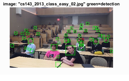
Results on class images

Results in a table

Analysis for variation ofparameters

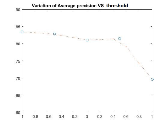
Variation of number of scales

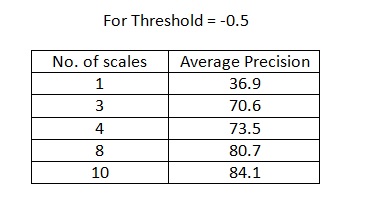
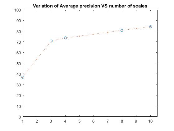
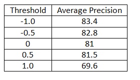
Number of scales=10, I varied the threshold and obtained the following results

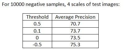
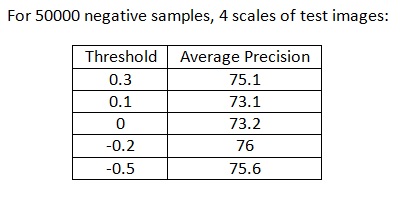
Number of scales=4, I varied the threshold at number of negative samples 10000 and 50000 and obtained the following results

EXTRA CREDIT

Extra Credit Part 1-Hard Negative mining

The average precision obtained over several runs is comparable with and without hard negative mining. There is no noticeable difference between the two.

Average precision without hard negative mining : 83.1

Average precision with hard negative mining : 83.2

Average precision with hard negative mining and lower threshold : 83.7

Extra Credit Part 2-Alternative Positive Training Data

The average precision with non augmented training set is: 81. The average precision with augmented training set is also comparable. Different runs give a minor improvement over the non augmented set.

NOTE: All average precision values are in percentage.