Project 5 / Face Detection with a Sliding Window
Goal: detect faces in images
Algorithmic Approach:
Getting Positive and Negative Features:
Positive and negative samples must be collected in order to train our classifier properly. For postive features, hog features are obtained for each image and then reshaped into a 1xD vector placed in a corresponding results matrix. For negative features, it is a bit more tricky. Random slices of the image are generated before obtaining hog features. These hog features are then stored in a similar manner to the positive features.
Training the classifier:
Here, one matrix combining the two feature sets was created in addition to a "labels" matrix. This labels matrix mirrors the combined features matrix in dimension, and it gives positive features a +1 and negative features a -1 for each spot in the original matrix. The transposes of each of these matrices, along with a lambda value, is then passed into an svm training function.
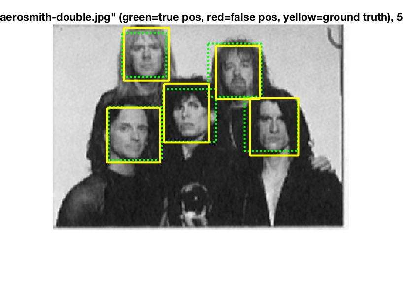
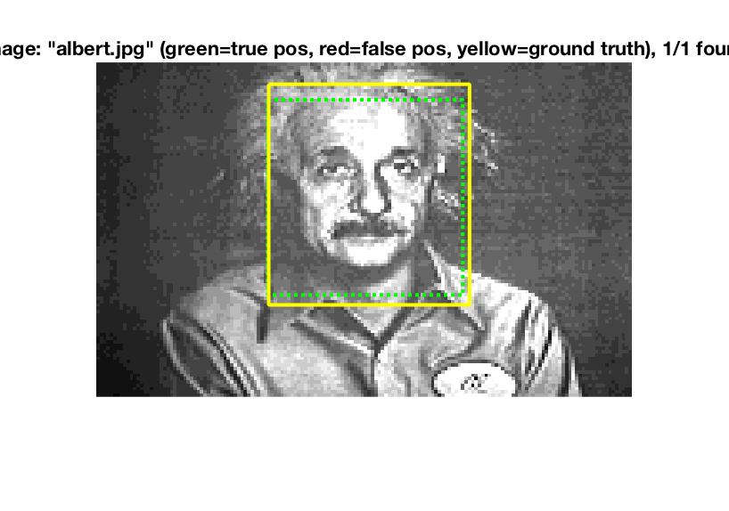
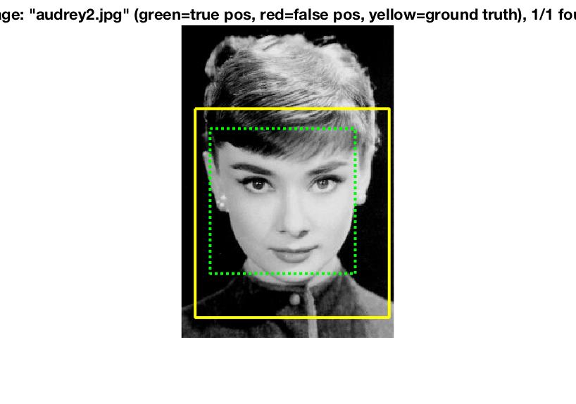
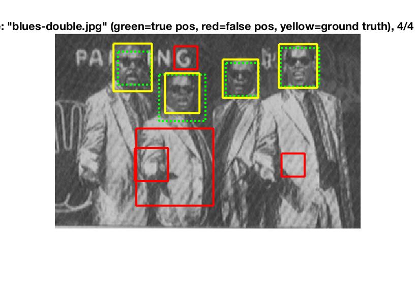
Run detector
Run detector is the most complex aspect of the algorithm. The idea here is to create a sliding window that checks for similarities of the window to the positive and negative features. Different windows are given different confidence ratings and then "bboxes" are stored in terms of the coordinates of said windows. Image ids are also stored along with this information.
The above algorithm is run at different scales to check for similarities at different image sizes. For this project, I decided to perform the algorithm at a 10% scale reduction each time.
Lastly, non-maximum suppression is run to remove duplicate detections.
Lambda experimentation:
Ultimately, a lambda of 0001 was selected. This got an accuracy of about 85%. However, lambdas of .001 and .01 had accuracies of about 81% or 82%. A lambda of .1 had an accuracy of 71%, and a lambda of 1 had an accuracy of 21%.
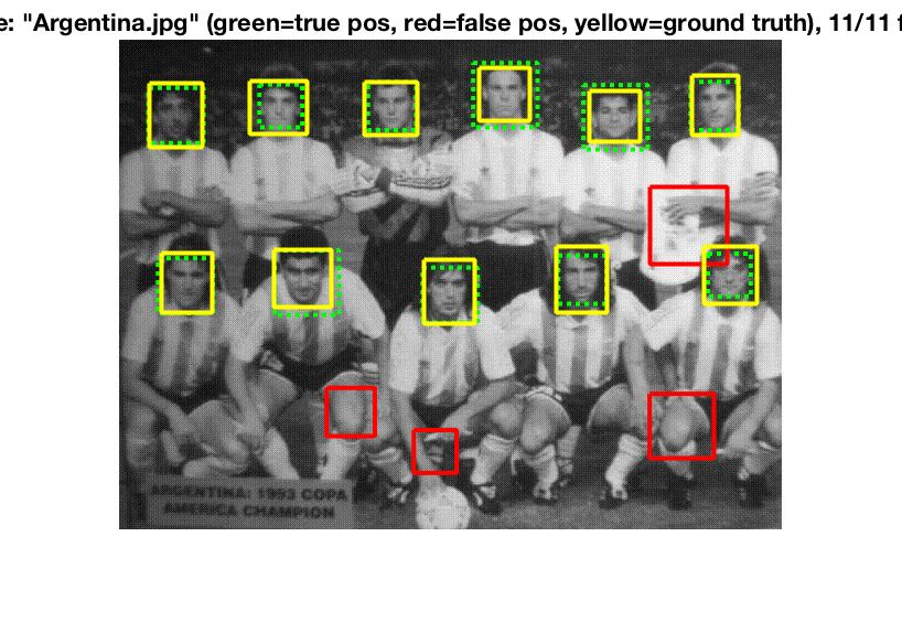
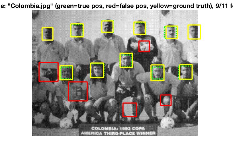
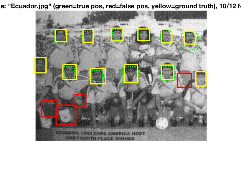
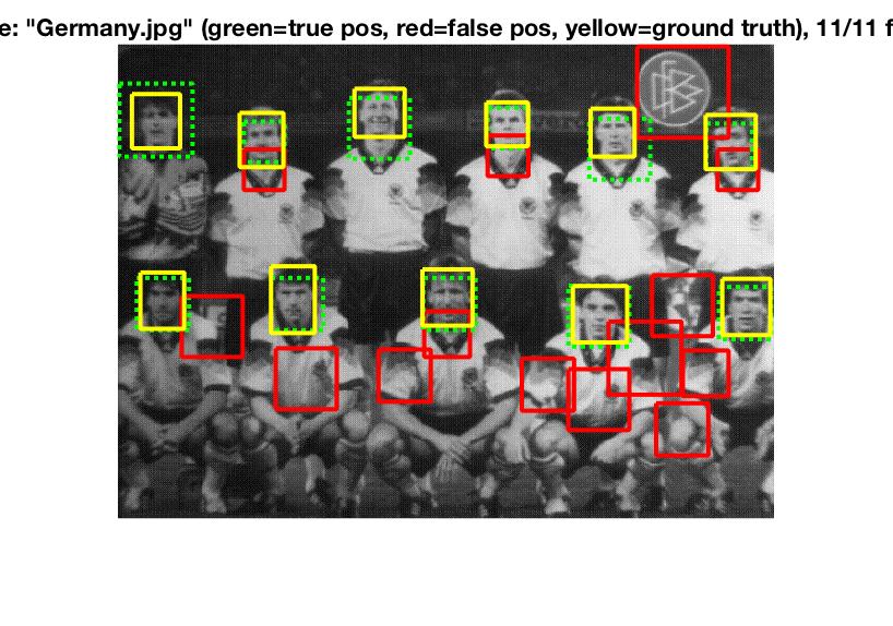
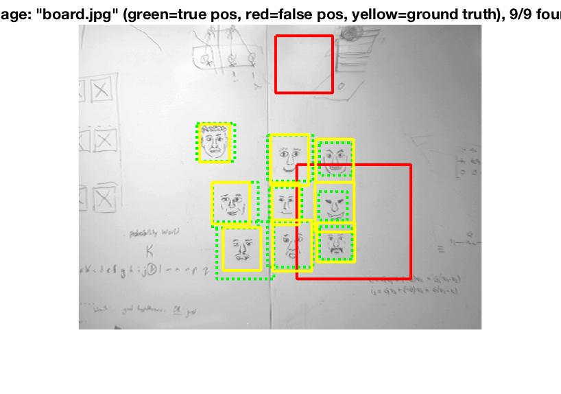
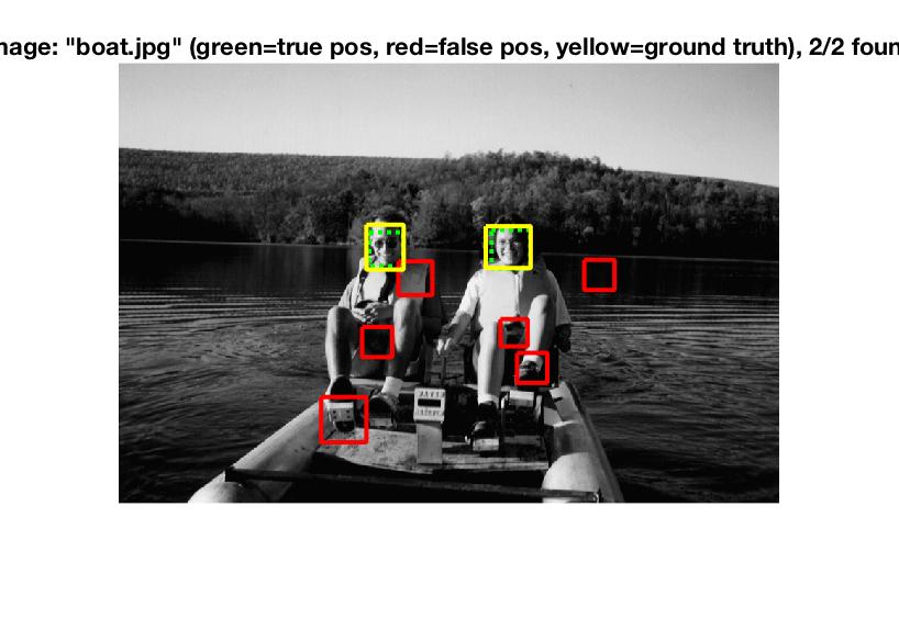
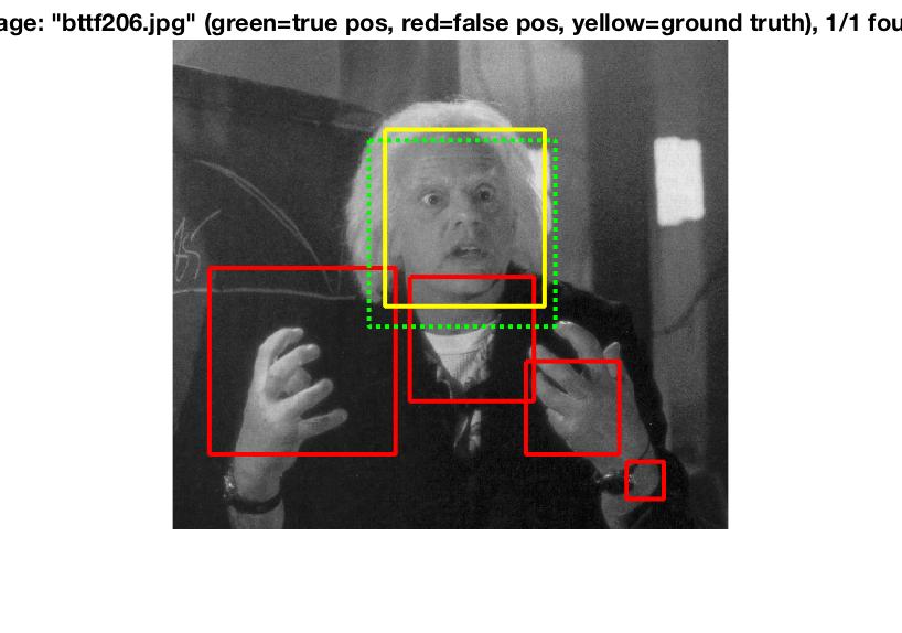
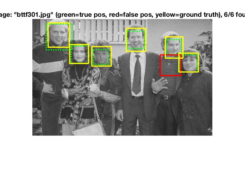
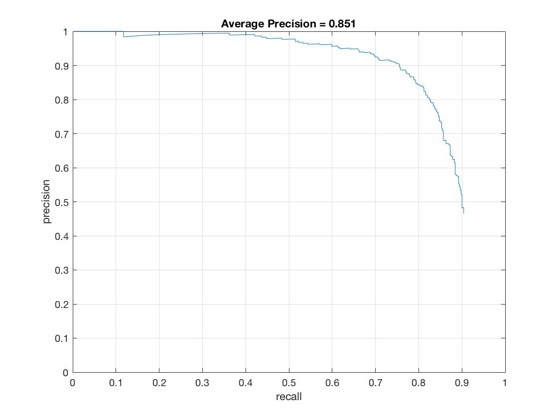 Precision for a threshold of .65 and a lambda of .0001.