Project 5 / Face Detection with a Sliding Window
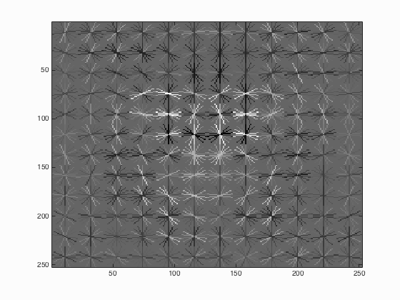
The HoG template for a 36x36 pixel face using 3-pixel cells. It slightly resembles a face pointed forward.
The general process of face detection with a sliding window is as follows:
- Generate positive and negative features from images with and without faces, respectively.
- Train a linear classifier to recognize positive features.
- Detect faces by using a sliding window and doing the following on each window of the image:
- At the current window, get a feature the same dimensions as the training features.
- Use the linear classifier to determine if the feature represents a face.
- If the classifier returns a confidence greater than some threshold, record the bounding box and confidence as a face.
- Remove duplicate bounding boxes from the results of the detector.
The resulting bounding boxes determine the location of a face in the input image. To evaluate a detector, we test on the CMU+MIT set of images, which include ground truths. Our metric of how well a detector is performing is the average precision on this set of images. A detector which is performing well should expect an average precision greater than 0.900. Throughout this pipeline there are several places where free parameters may be adjusted. These free parameters may have large implications in the final average precision of our detector. I will go into each one of these steps and examine the reasoning behind the decisions made.
Extracting Features
The first step of the pipeline is to extract features from both images with and without faces. The idea behind these are similar. First, take crops of the image as defined by a template size. Next, compute a Histogram of Gradients (HoG) over this crop, and store this into a 1-dimensional vector. This vector is the features we will use to train our linear classifier. An example of a rendered HoG feature is shown at the beginning of this page. Finally, repeat this process over thousands of images to collect all of the features. Two obvious free parameters are present when extracting features. First is the template size and second is the cell size of the HoG features. For collecting positive features, the Caltech Web Faces project provides 6,713 cropped 36x36 faces. For this reason, the template size remains at 36x36 for the entirety of this project. As far as the cell size, a indirect correlation was found between it and the final average precision, up to a point. More information about this relationship will be analyzed later on. Finally, this step was moderately quick when compared to the entire time used for the pipeline. Extracting positive features took between 10 and 18 seconds, whereas negative features only took around 6 seconds for approximately 10,000 samples. The exact process has some minor differences between the positive and negative feature extraction.
Positive features
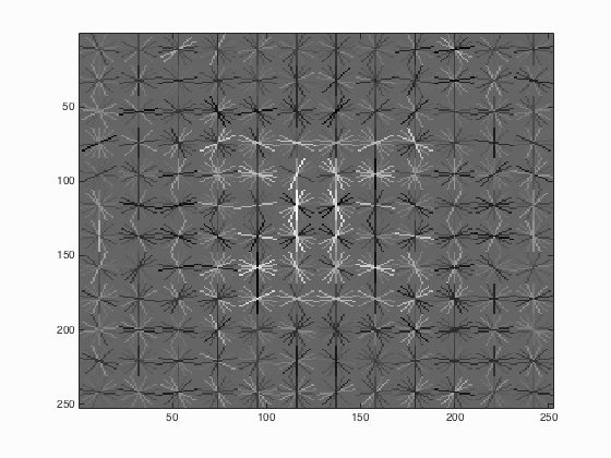
Since the input images are already at the desired template size, cropping the image to any degree is not necessary. Therefore, we can simply compute the HoG feature across the entire image to get the resulting feature. At this stage of the pipeline, we may augment the training data by reflecting and warping the original images for additional features. To do this, we may simply flip the x or y dimensions to create mirrored or flipped images, respectively. After performing these operations in all combinations, the amount of positive training data is quadrupled. You can see the resulting HoG render to the right. Immediately, it is obvious that the render does not resemble a face as much as the HoG render above. My original expectation was that augmenting the data with these image warps would result in an improved performance. The final results indicated a larger number of false positives and a dip in average precision by approximately 5%. I assume the increased number of false positives was a result of the facial HoG template being too generic and not properly representing the set of faces seen in the testing data. Some changes which were considered include only augmenting the training data with a portion of reflected faces as opposed to reflections of every face. Based on this analysis of feature extraction, for the best obtained average precision, the feature augmentation was removed from positive feature extraction.
Negative features
The given set of images to extract negative features don't contain any faces.
Because of this, any random crop of the template size is guaranteed to not match a feature with a face.
One special input parameter to the negative feature function was the number of samples desired.
This parameter is not included for getting positive features since each face will eventually become one or more features in the training data.
In order to determine how many features to collect per image, a certain number of random crops were found from each image.
To be exact, the number per image was floor(num_samples / num_images), where num_samples is the parameter passed in and num_images is the number of images used to train.
The floor function simply rounds the resulting floating precision number down to an integer.
This process results in negative features of the same dimension as the positive features since they use the same template size and HoG cell size.
Since this process uses floor rounding, the number of features returned may be slightly less than the desired number of samples.
Changing this to ceil rounding results in slightly more features, however no impact on final performance was noticed.
Linear Classifier
For this project, a support vector machine was used as the linear classifier. Due to the simplicity of a linear classifier, this step outperformed the rest of the pipeline in terms of accuracy and time. The obvious free parameter is lambda, the training margin. Modifying this value has an impact on training accuracy, although not to a large degree. Since the accuracy measured is training accuracy, it was almost always found to be extremely high. When lambda was set to the recommended 0.0001, training accuracy was found to be 0.999+. By adjusting this up to 0.1, training accuracy only dipped to 0.996, however the impact on the final average precision was a 5% drop. Finally, with a value of 10, training accuracy and average precision dropped to 0.598 and 0.000, respectively. With this last result, the linear classifier was very unstable, blindly classifying everything as negative. Based on this analysis, the optimal value of lambda was found to be 0.0001.
Facial Detector

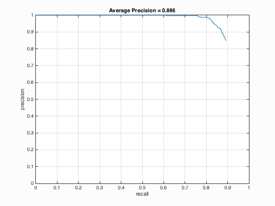
A multiscale detector's precision-recall curve using HoG features with 3-pixel-cells.
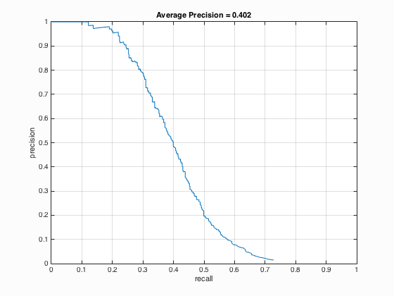
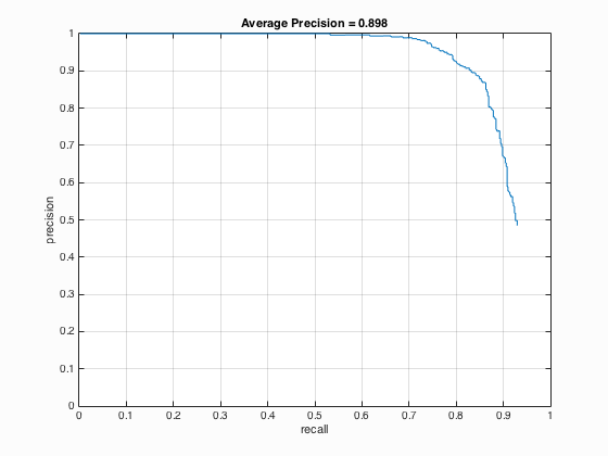
As outlined above, the process for detecting a face in an image is fairly straightfoward. You create a sliding window the size of the template, 36x36 in this case, and apply the linear classifier to the current window. To speed this process up, the entire image is transformed to the HoG feature space and the sliding window steps by the cell size number of pixels each iteration. With this process, a smaller HoG cell should slow execution speed considerably, but also increase the average precision. The first parameter is the threshold to determine if a window is a face. For debugging, this value was set to be low, approximately -2.0, resulting in an average precision of 0.402. This performance is not sufficient, as it missed a large number of true positives and returned many false positives. In order to drastically improve the average precision, multiscale detection had to be implemented. The idea behind multiscale detection is simple: perform detection on an image at a certain resolution, then downsample the image by a fixed factor and perform detection again. Continue to repeat this process until a fixed number of scales have been searched, or the image is too small to process. For my implementation, I opted for the latter. Specifically, whenever one of the dimensions of the currently scaled image was less than the template size, I stopped execution and returned the resulting bounding boxes at multiple scales. Multiple scaling factors were tested, and a balance between execution time and average precision was found to be at 0.90. That is, at every iteration, downsample the image to 90% of the current version. This one change was the largest improvement when compared to any other modification, however the threshold had to be increased from -2.0 to 1.0 in order to reduce the number of false positives. With this configuration, the average precision achieved was 0.858. Finally, the bounding boxes for each image were compared and duplicates were removed whenever the centroid of two bounding boxes overlapped, in which case the most confident box was kept. When the HoG cell size was decreased from 6 pixels to 4 pixels, the average precision increased by 4% to 0.898. When the HoG cell size was further reduced to 3 pixels, the average precision of 0.886 was found. After tuning the threshold to increase average precision at the expense of more false positives, the best value was found at 0.922 using a threshold of 0.6. Unfortunately, the detection algorithm's runtime suffered noticeably whenever the HoG cell size decreased, ranging from 65 seconds at 6 pixels with multiscale detection up to a whopping 350 seconds at 3 pixels and multiscale.
Results
The best average precision discovered by the pipeline was 0.922. The precision-recall curve is shown in the previous section. These results were found using HoG templates of 36x36 pixels and 3-pixel cells. For positive features, the resulting HoG features were not augmented with any sort of image transformations. For negative features, 10,000 samples were evenly drawn among the training set of non-face images. The linear classifier was trained using a lambda of 0.0001. The detector used a threshold of 0.6 and scaled the images down by a factor of 0.9 each iteration. The detector stopped execution when the one of the dimensions of the current image was less than the template size. This whole pipeline ran for 582 seconds.
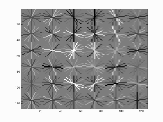
The HoG template for 36x36 pixel faces using a 6-pixel cells.
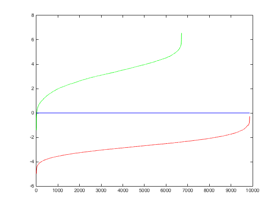
The training curve for the linear classifier using lambda=0.0001. This classifier had an accuracy of 0.999 on the training set.
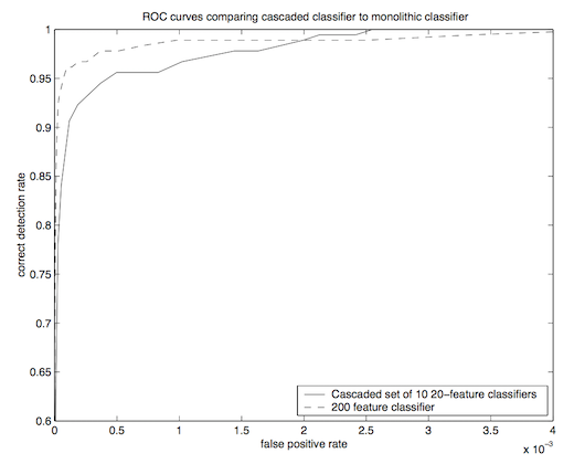
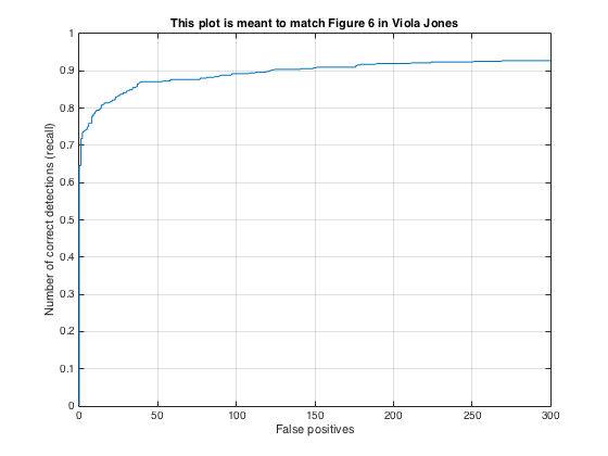
A graph from Viola-Jones 2001 showing the correct detection rate as a function of false positive rate. The left graph is from the original paper and the right graph was produced by my implementation. The solid line on the left graph and the blue line on the right graph share a similar trend, however the original paper has a higher average precision than what I implemented.
The precision-recall curve for a single scale detector using HoG features with 6-pixel-cells and a threshold of -2.0.
The precision-recall curve for a multiple scale detector using HoG features with 6-pixel-cells and a threshold of 1.0.

The precision-recall curve for a multiple scale detector using HoG features with 4-pixel-cells and a threshold of 1.0.
The precision-recall curve for a multiple scale detector using HoG features with 3-pixel-cells and a threshold of 1.0.
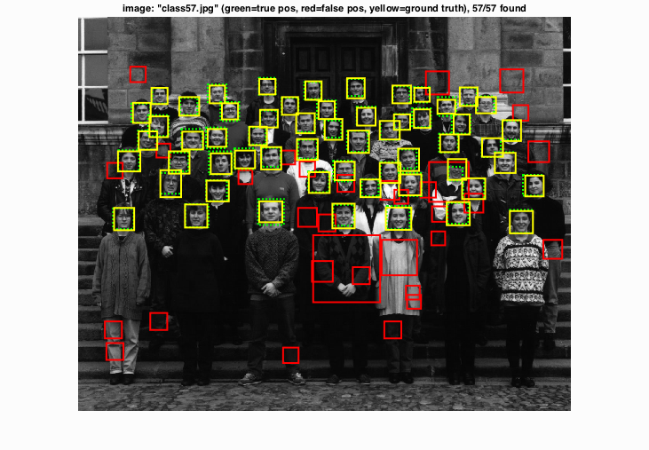
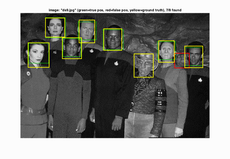
Following this are various images and their results I found interesting for whatever reason. This one contained many small faces.
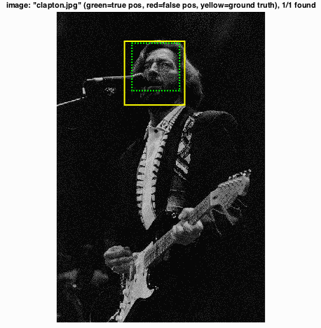
This one features a slightly larger face which is not directly front-facing and has some shading. Also, it's Slowhand.
This one identifies faces of multiple races. As to why I find this interesting, please see this Wired article. It appears it does struggle on other "species", however.
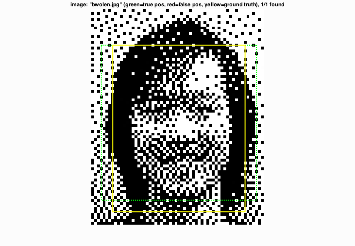
I can't say for certain what this image is, but it is either heavily post-processed or manmade. Either way, the detector still identifies the face.
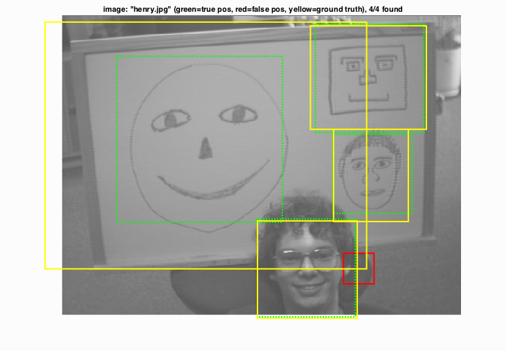
An artist's rendition of faces.
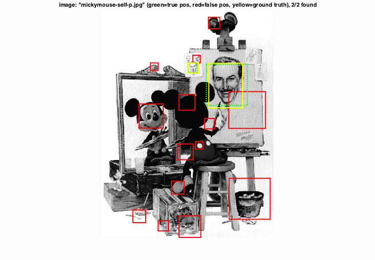
This one is interesting for several reasons. The detector identifies Micky Mouse as a face although it is not included in the ground truth. On the upper-lefthand corner of the canvas are three small faces of Walt Disney. Only one of them is included in the ground truth, however the detector identifies a second one as a positive.
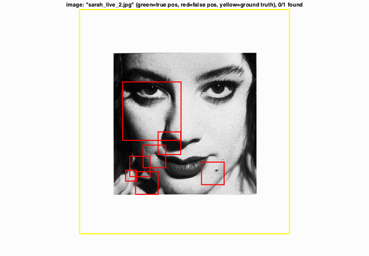
When the face takes up the entire photo, the detector seems to underperform. This may be fixed by first scaling the image up some before performing the standard multiscale detection algorithm.