Project 5: Face detection with a sliding window
Data
In order to develope the Facial detection algorihtm, I used facial Caltech Web Faces Project and Scenes from the SUN scene database and Wu et al paper. The combined CMU+MIT test set was used to test the accuracy of our facial detection algorithm.
For my ground truth set, I used 6713 36x36 cropped faces from the Caltech Web Faces project. and randomly sampled 36x36 patches from the scene photos to get my negative examples.
I also mined hard negative examples from the scenes by running a trained SVM model on the scene photos and recording the false positive examples though this was not particularly effective.
Facial Detection Algorithm
I used a machine learning method to detect faces in photos with a sliding window algorithm.
There were 4 main steps to the basic algorithm, obtaining the Positive and negative image samples, encoding the features into SIFT like scale invariant HOG features, training a classifier based on the training examples, and then testing on the testing set using the classifier and a sliding window algorithm on the images HOG features.
As stated previously, 36x36 patches were taken to create the positive and negative training sets. All photos were converted to black and white and pixel values were normalized to 0-1. I used HOG features to encode the images. These features are scale invariant so it becomes easy to allow the final algorithm to detect faces of different sizes though we trained the classifier on all 36x36 faces. We tried a 3,4, and 6 cell size for the HOG features.
Afterwards, I tried training a SVM, Decision Tree, and KNN classifier with the training data. The KNN classifier quickly proved to be too slow for realistic use and the SVM classiffier was the most effective. More details on the Decision Tree are below.
Decision Tree results
The Decision tree was fast, but had difficulty since it could not give me a good confidence measure and thus suffered from a very high false positive rate since it's decision boundaries were mostly binary so threshold tuning proved difficult. Below is a graph of the precision vs recall of the Decision tree classifier on the testing dataset with varous thresholds compared the same graph with the SVM classifier. As you can see, though high recall is possible, the precision drops incredibly quickly and thus, it is quite useless for this task.
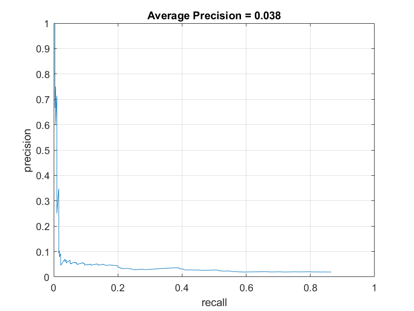
Decision Tree with HOG cell size of 6 |
Gaussian Blur with HOG cell size of 6 |
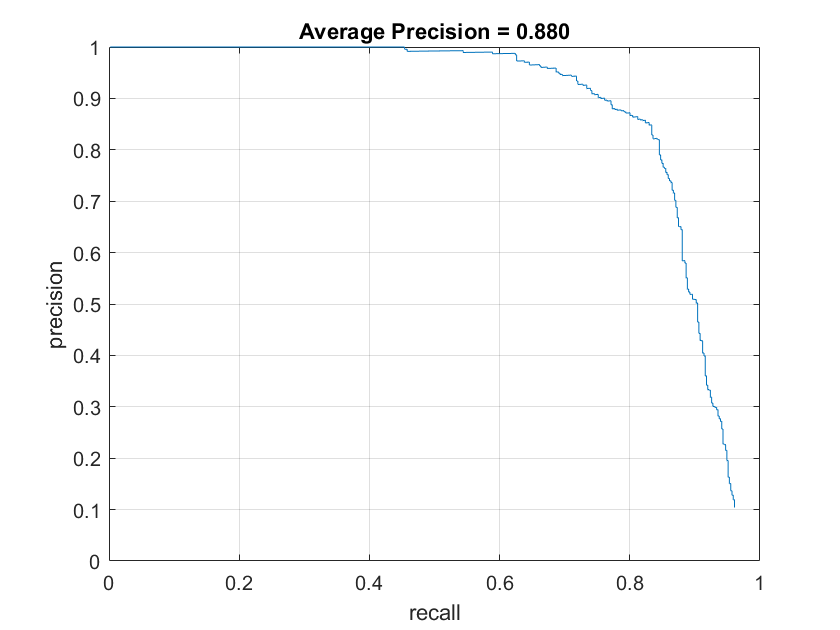
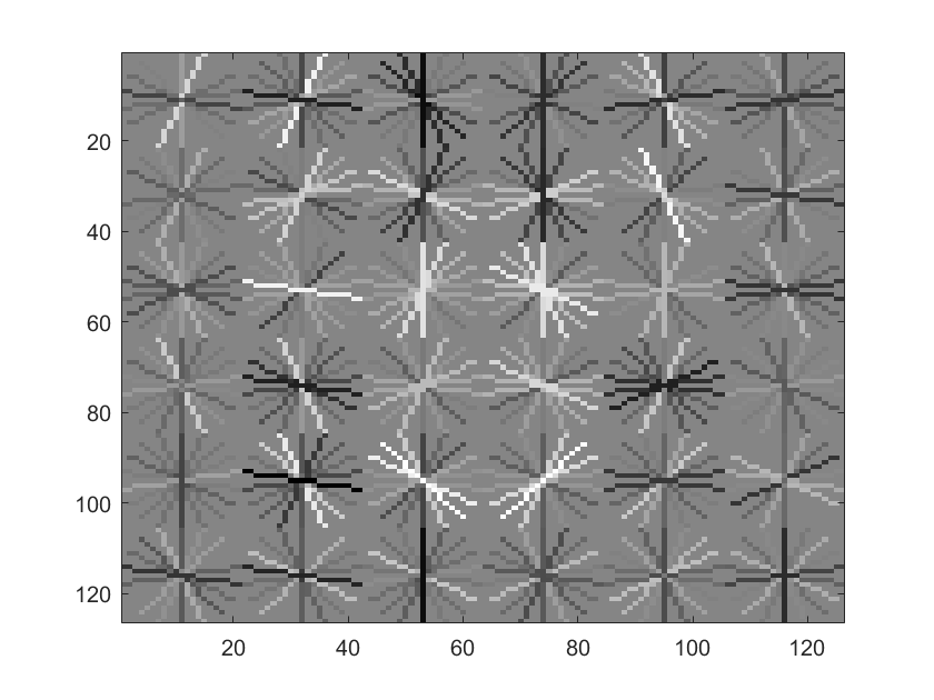
The SVM on the otherhand, had relatively high precision and was pretty good at differntiating faces. This can be seen in a visualization of the HOG features the SVM detected as shown below. As can be seen, a vaguely face shape can be differentiated.
The sliding window algorithm
The method used on the testing set was a sliding window algorihtm with multiple scales of detection. First, the image was converted into HOG cells. We tried different cell sizes 3, 4, and 6. Then each window of 6x6 HOG cells was classified using the classifier and a score was retrieved. If the score was high enough, the possible face was recorded. Then the image was scaled down 90% and the same process was repeated. Then the image was scaled down again and again until it was too small for a 36x36 pixel window to fit. A non-maximal suppression was used to handle duplicate and overlapping classifications.
Different HOG Window Sizes
We tried different HOG window sizes, and the smaller windows tended to become more accurate. This makes sense, since the resolution of the face in HOG pixels becomes greatly larger. This can be qualitatively seen in the comparative humaness of the visualizations below.
|
SVM visualization with HOG cell size of 6 |
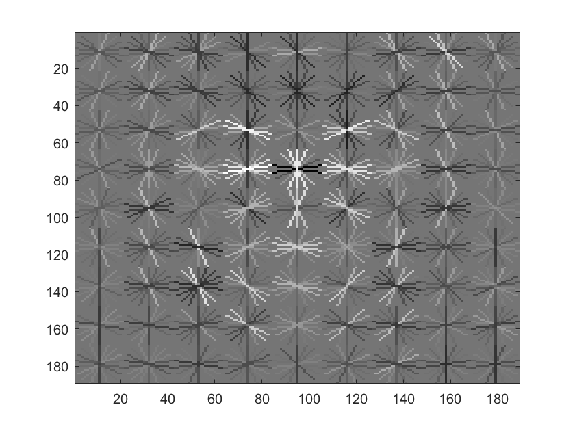
SVM visualization with HOG cell size of 4 |
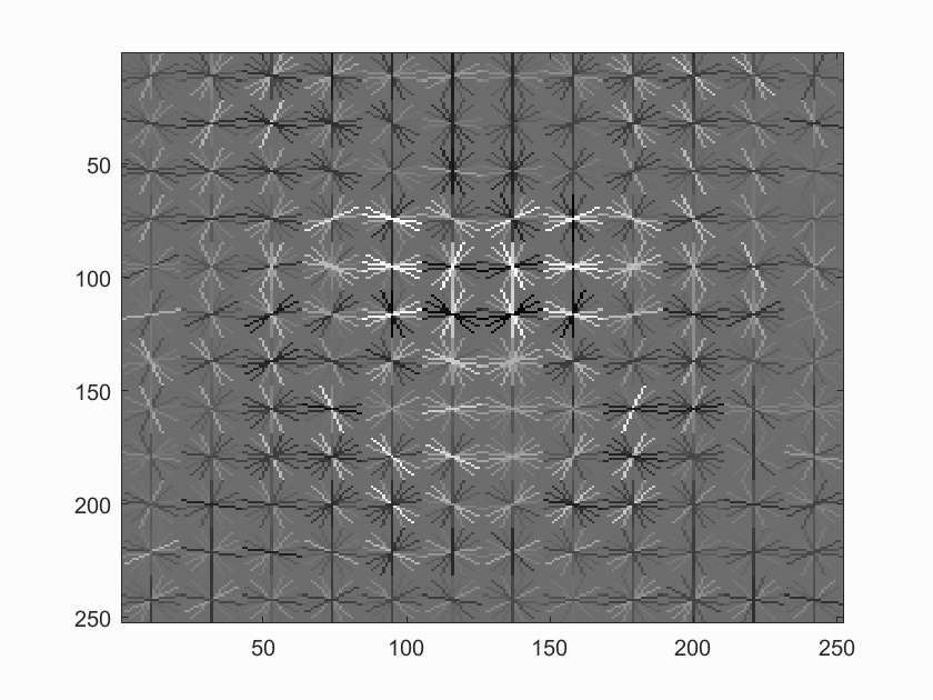
SVM visualization with HOG cell size of 3 |
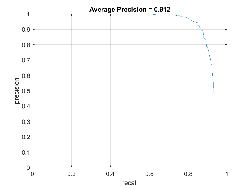
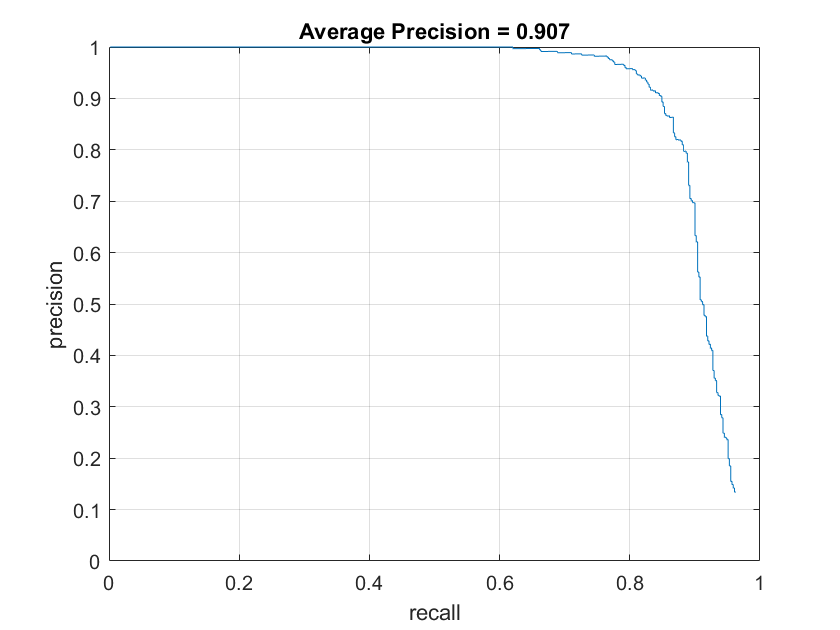
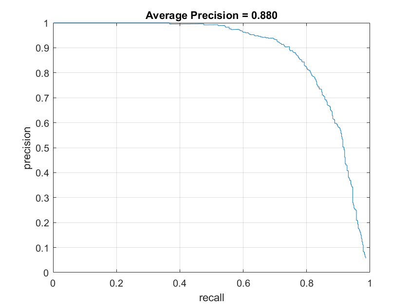
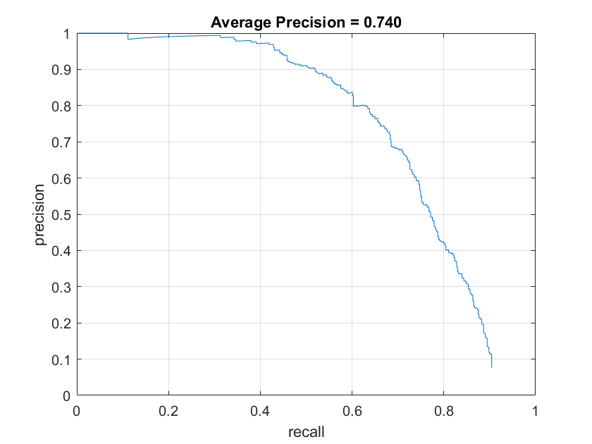
Below are the accuracy graphs with the different HOG cell sizes on the SVM model. The increasing average precision quantitatively show the increasing accuracy with small cell sizes.
|
SVM Accuracy with HOG cell size of 6 |
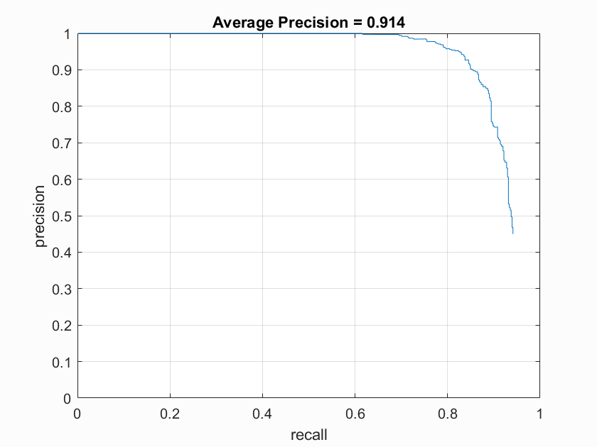
SVM Accuracy with HOG cell size of 4 |
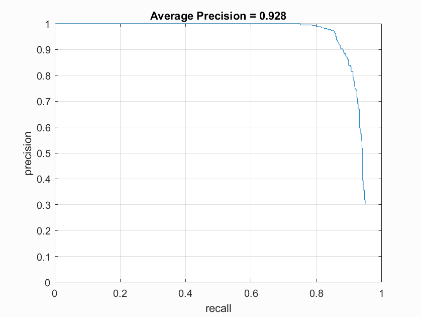
SVM Accuracy with HOG cell size of 3 |
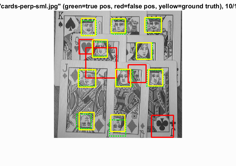
Below is an example of a test image with faces recognized by the SVM detector
|
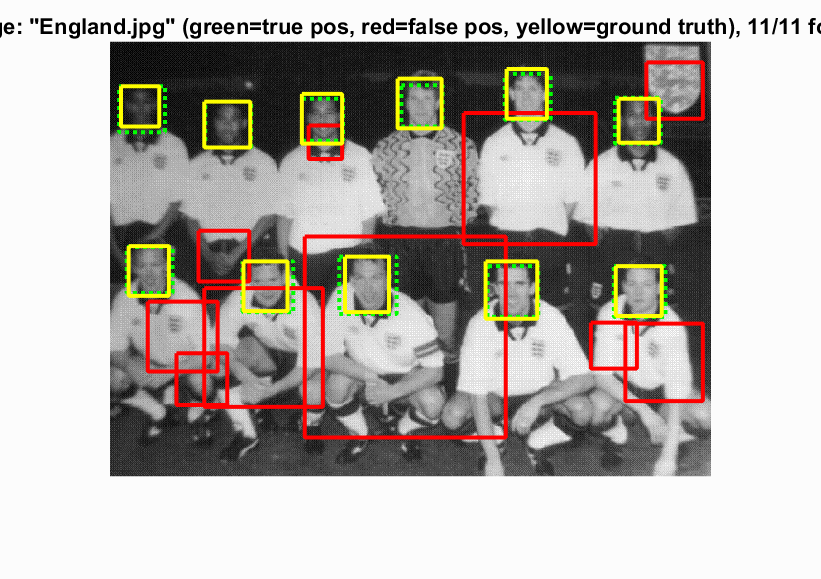
|
Mining Hard Features
I tried mining hard features in order to try to increase the accuracy. I mined them by running the svm classifier on scene data and recording the false positives. Unfortunately, this method did not bring good results and always lowered accuracy. I attemped this with 1000 and 5000 negative examples and it still never increased accuracy. I believe this is due to the fact that the type of near face examples is too rare in images and that the false positives likely were near facial features in the scene. It can be seen in the visualizations that the hard negatives greatly changed the SVM model learned.
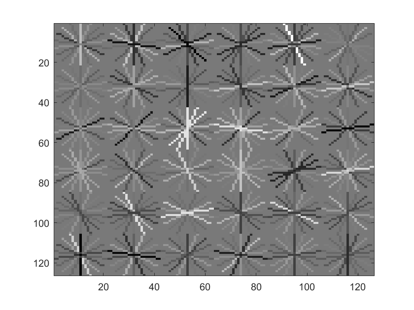
SVM of size 6 and 1000 examples |
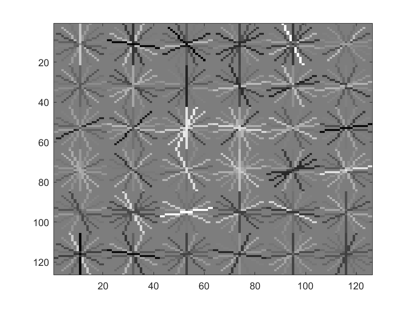
SVM with Hard negative of size 6 and 1000 examples |
SVM accuracies with size 6 with 5000 examples |
SVM with Hard negative of size 6 and 5000 examples |
SVM accuracies with size 6 with 1000 examples |
SVM with Hard negative of size 6 and 1000 examples |