Chenkai Shao

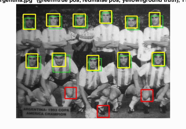
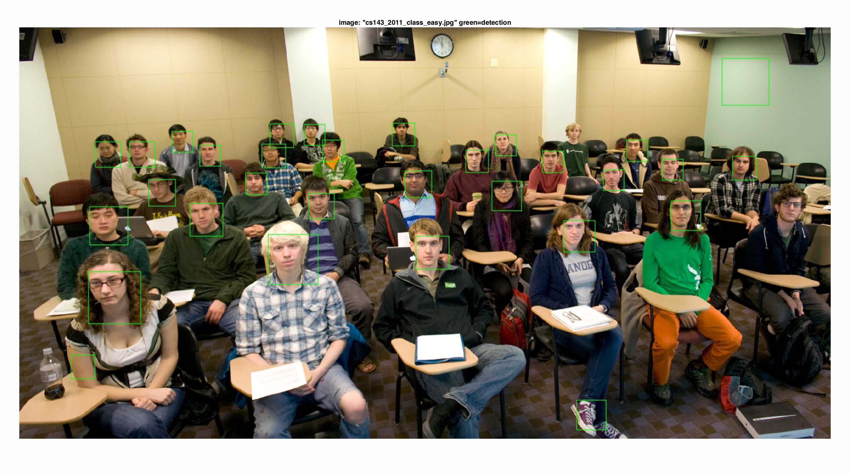
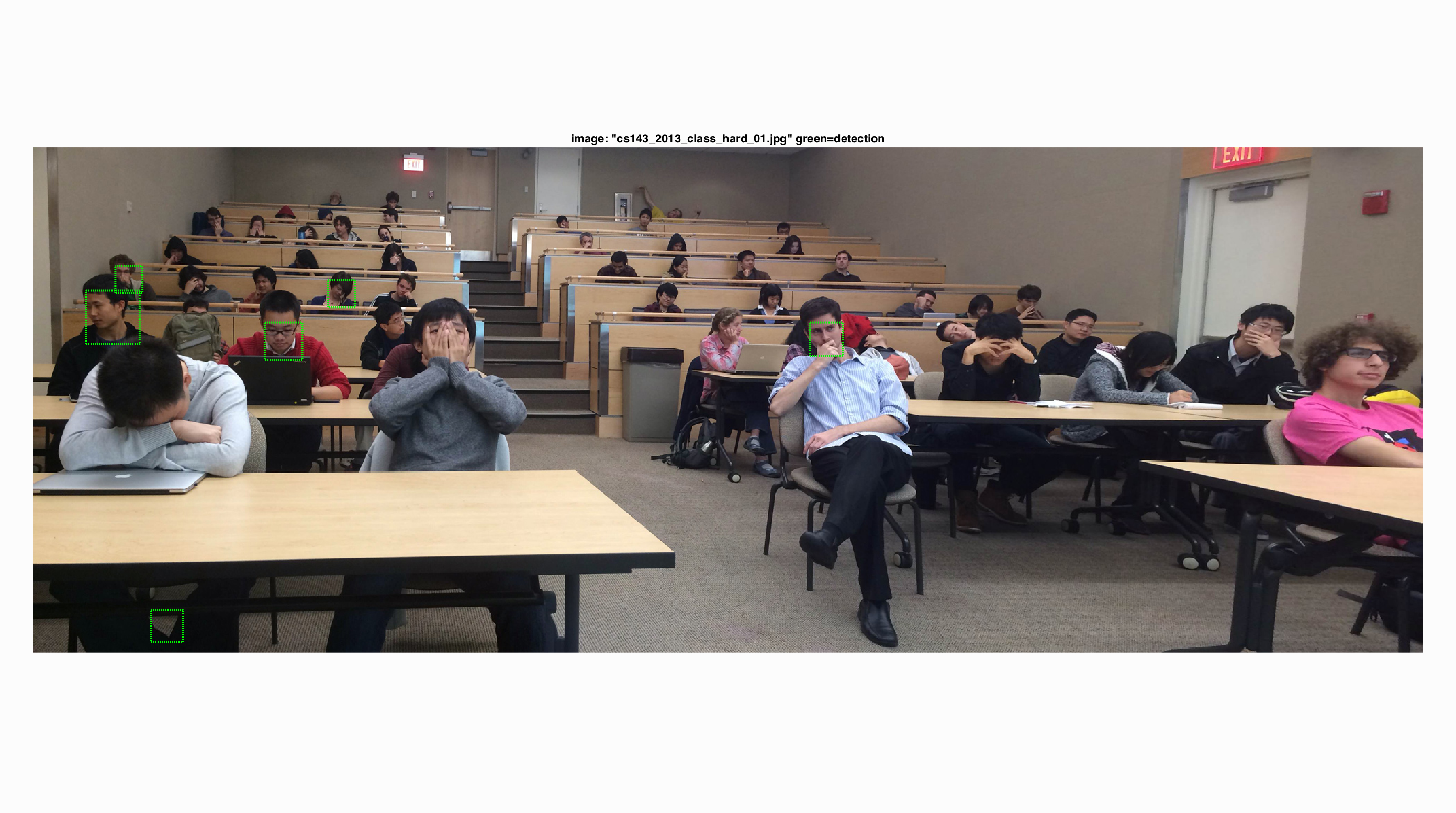
Example result of face detection.

Get HOG features

For the 36 x 36 image crops with positive features, I simply use the vl_hog function to get the HOG features for each image crop. For the random negative image samples, I randomize three parameters: the image id, the downsampling scale and the position of the 36 x 36 patch. The scale ranges from feature_params.template_size / min(size(image)) to 1 in that the downsampled image has to be at least 36 x 36.

Train a classifier

I use the vl_svmtrain function to train an SVM that classifies if an image patch represents a face. The SVM is trained with the HOG features obtained in the previous step. An important parameter here is the lambda, which controls the amount of bias. I test different lambda with the same training data and all other parameters fixed.

Lambda	Average Precision	False Positive
0.01	0.813	150
0.001	0.827	160
0.0001	0.843	more than 300
0.00001	0.857	more than 300

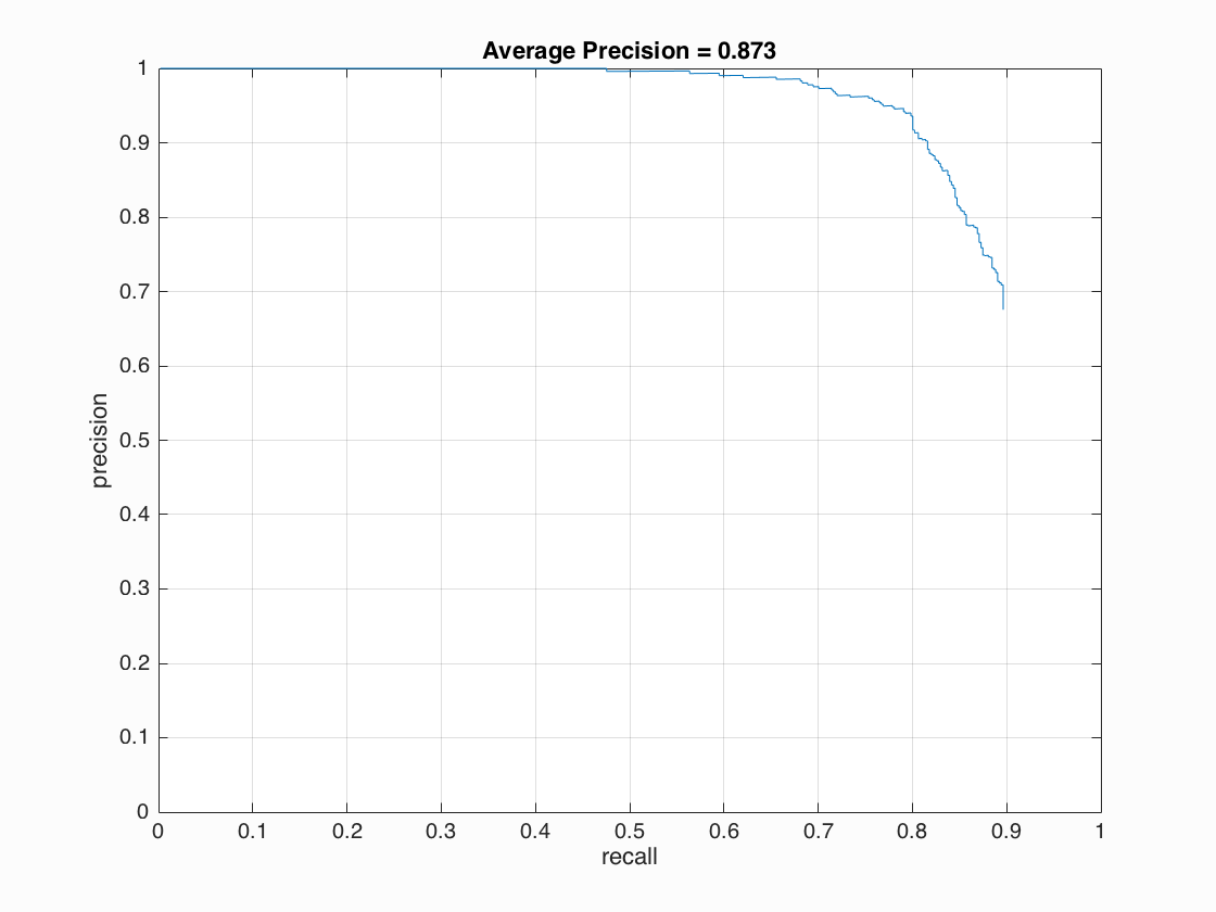
From the table above, we can see that 0.001 has a decent average precision and a reasonable amount of false positive.

Face detection

For each test image, I run the detector on different downsampling scales and use max suppression to remove the duplicate detections of different scales.

The scale step is an important parameter. I downsample the image by a scale of 0.95 in every loop recursively. For example, the size of the downsampled image is 0.95 * original size in loop 2 and 0.95 ^ 2 * original size in loop 3. A smaller scale reduces the amount of computation whereas a large scale finds more faces and also increases the false positive rate. From my experiment, 0.95 is the best number for this parameter. A scale larger than 0.95 increases the computation time and does not increase the average precision much.

For each downsampled image, I run vl_hog on the whole image and get an array of HOG cells. Then I use a sliding window of 6 x 6 HOG cells and step the sliding window by 1 HOG cell. I run the SVM classifier on the sliding window and register the window as face if the classifier output is larger than a threshold.

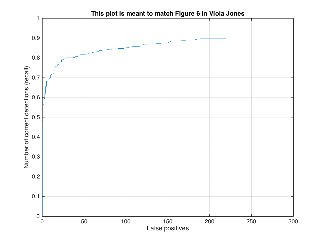
The threshold is the most interesting parameter to play with. It controls how strict the detector filters out non-face detections. It is a tradeoff between recall rate and false positive rate. A higher threshold passes less detections and thus produces less true positive and false positive. A lower threshold does the opposite. The goal is to find more true positive and less false positive. From experiment, I find 1.75 is the best threshold, which gives around 0.83 average precision and 150 false positive. I can always get better average precision if I use a lower threshold such as 1 but the false positive rate will be too high. If I use 2.25 as the threshold, I can get 75 false positive but I can only get around 0.79 average precision.

Code that runs the classifier on different sliding windows and different downsampling scale

    while min(size(image)) >= feature_params.template_size
        HOG = vl_hog(single(image), feature_params.hog_cell_size);
        
        for row = 1 : size(HOG, 1) - feature_params.template_size / feature_params.hog_cell_size + 1
            for col = 1 : size(HOG, 2) - feature_params.template_size / feature_params.hog_cell_size + 1
                HOG_win = HOG(row : row + feature_params.template_size / feature_params.hog_cell_size - 1, col : col + feature_params.template_size / feature_params.hog_cell_size - 1, :);
                HOG_win = reshape(HOG_win, 1, D);
                confidence = HOG_win * w + b;
                if confidence > 1.75
                    cur_x_min = floor(col * feature_params.hog_cell_size / scale);
                    cur_y_min = floor(row * feature_params.hog_cell_size / scale);
                    cur_bboxes = [cur_bboxes; cur_x_min, cur_y_min, cur_x_min + floor(feature_params.template_size / scale), cur_y_min + floor(feature_params.template_size / scale)];
                    cur_confidences = [cur_confidences; confidence];
                    cur_image_ids = [cur_image_ids; test_scenes(i).name];
                end
            end
        end
        image = imresize(image, 0.95);
        scale = scale * 0.95;
    end

Results in a table

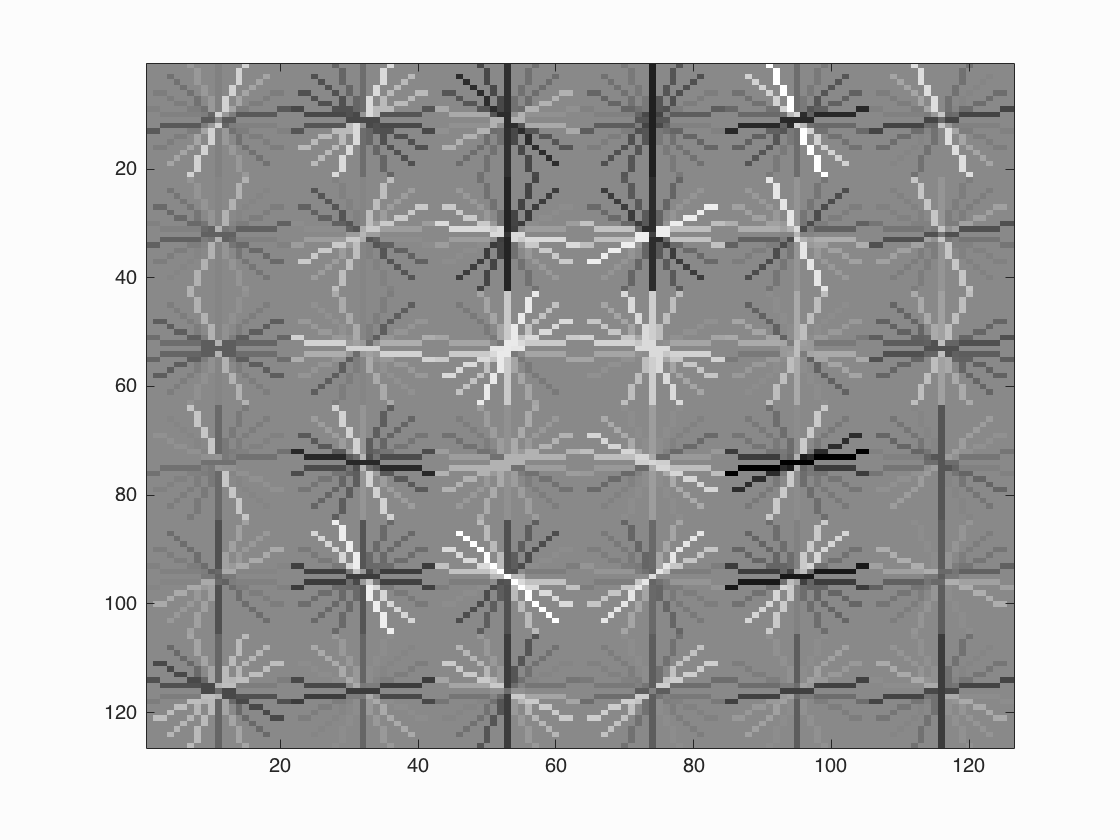
Face template HoG visualization.

Precision Recall curve.

False Positive curve.

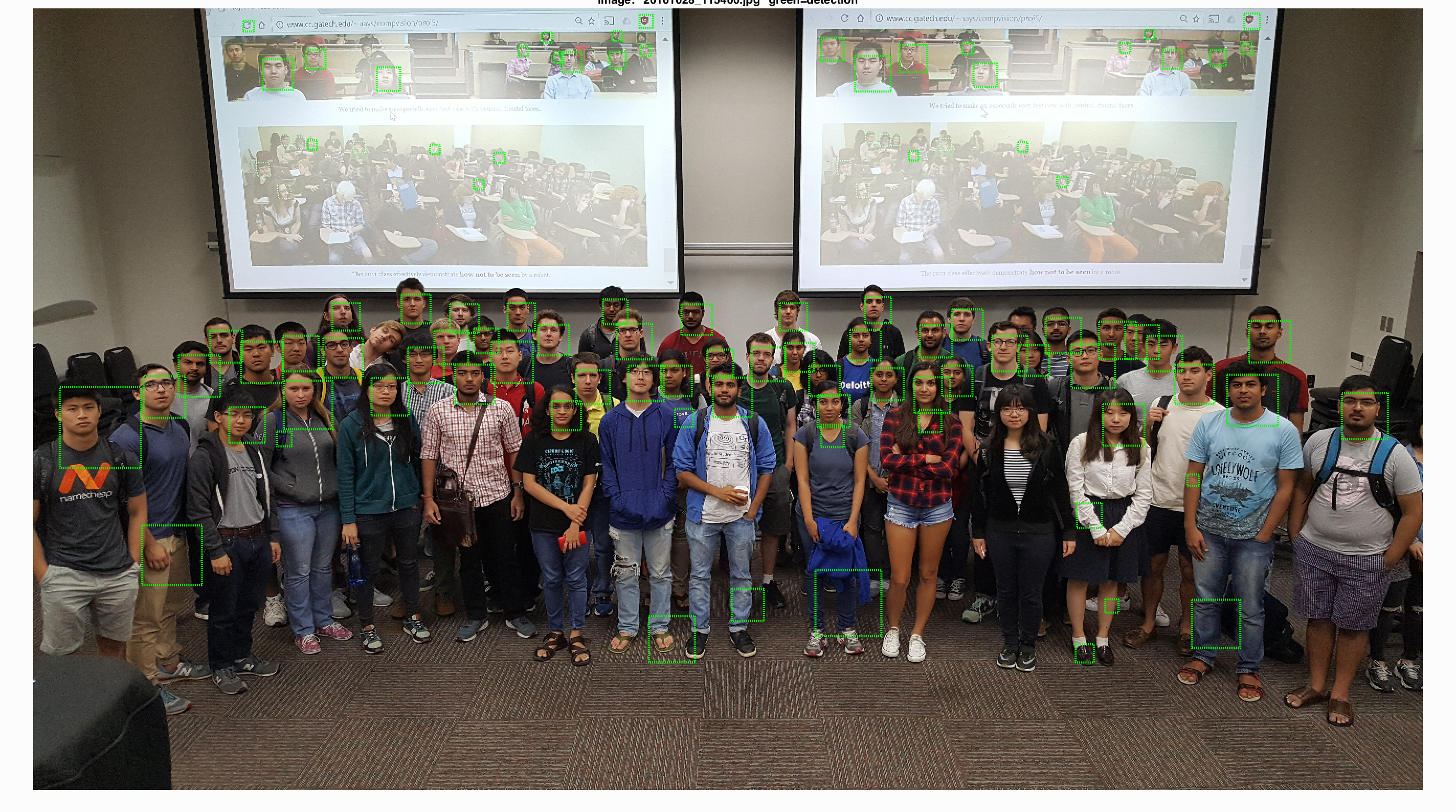
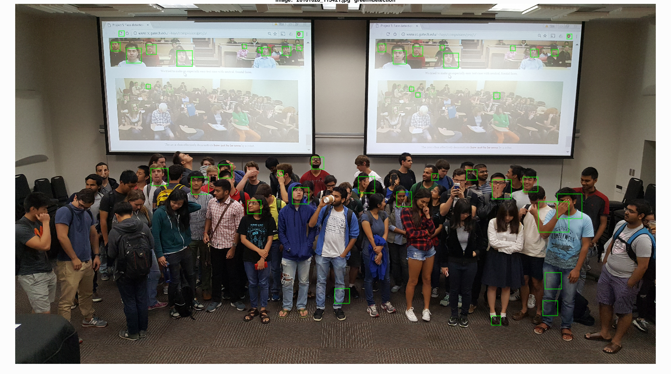
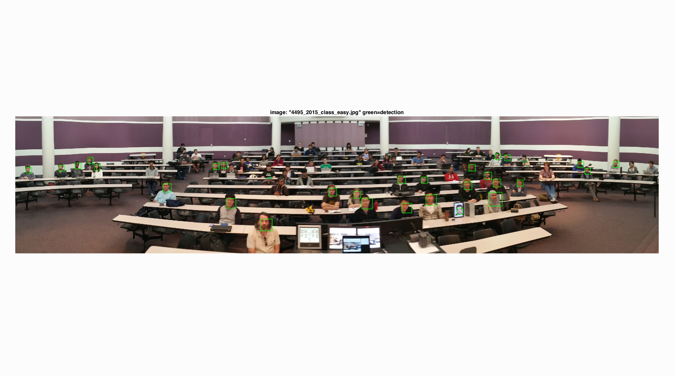
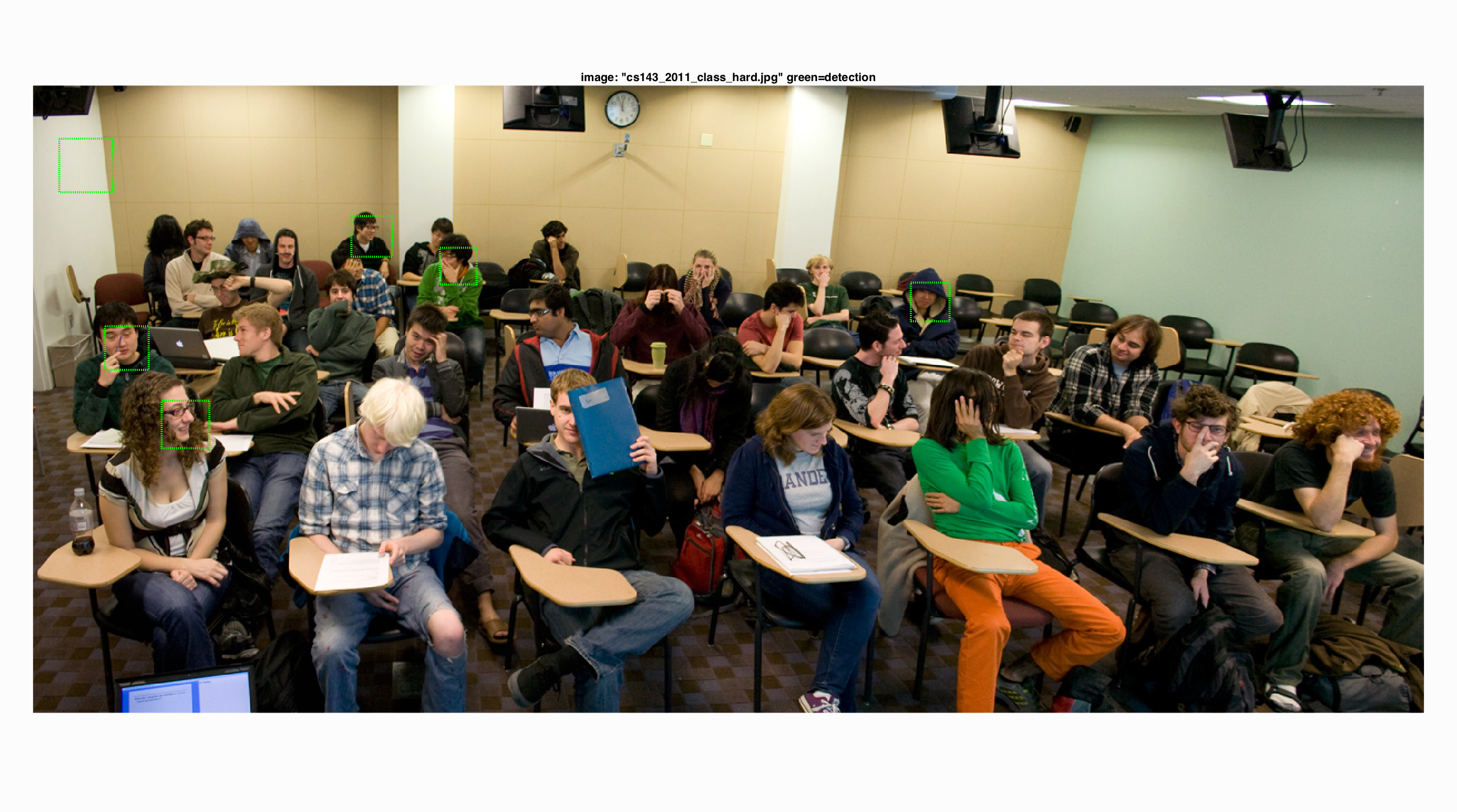
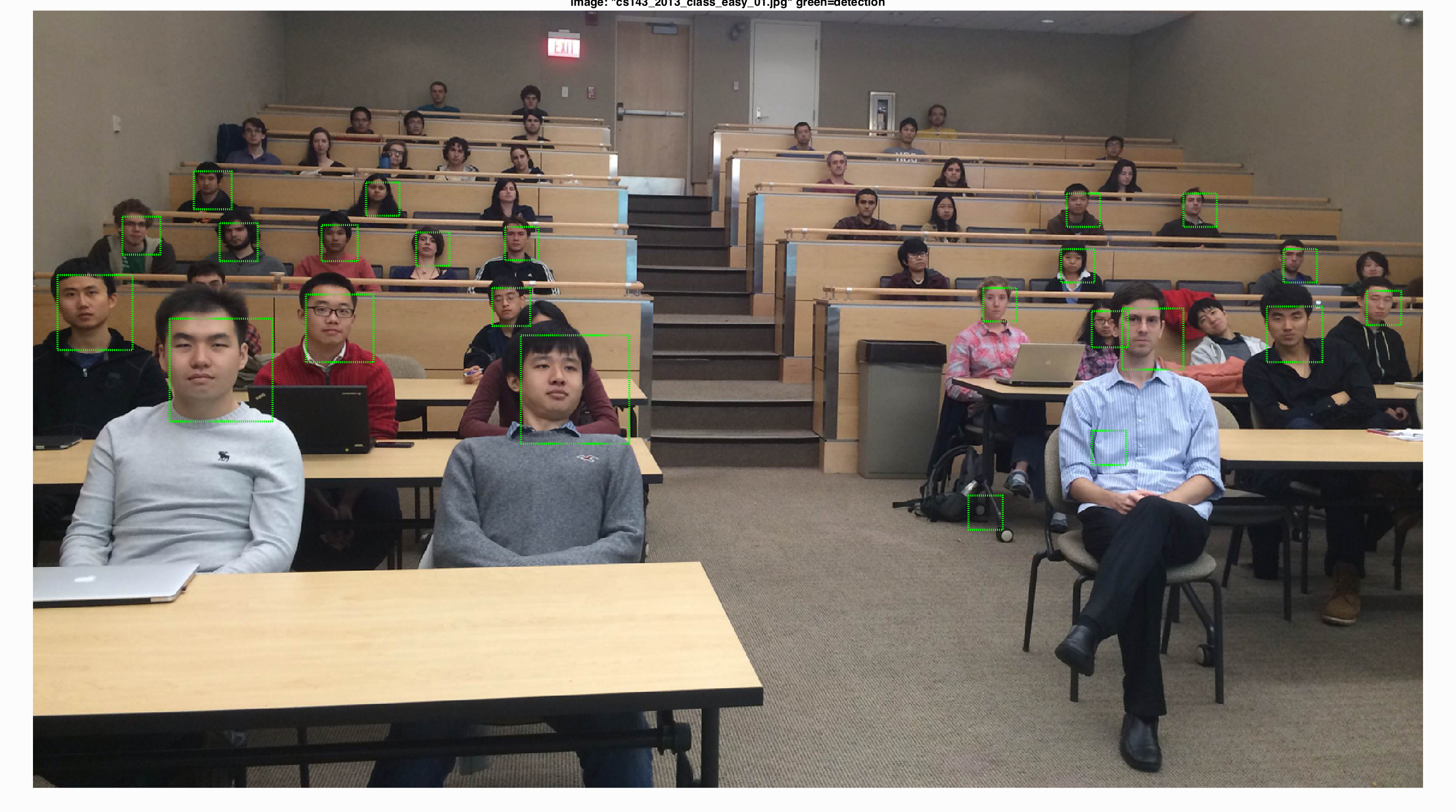
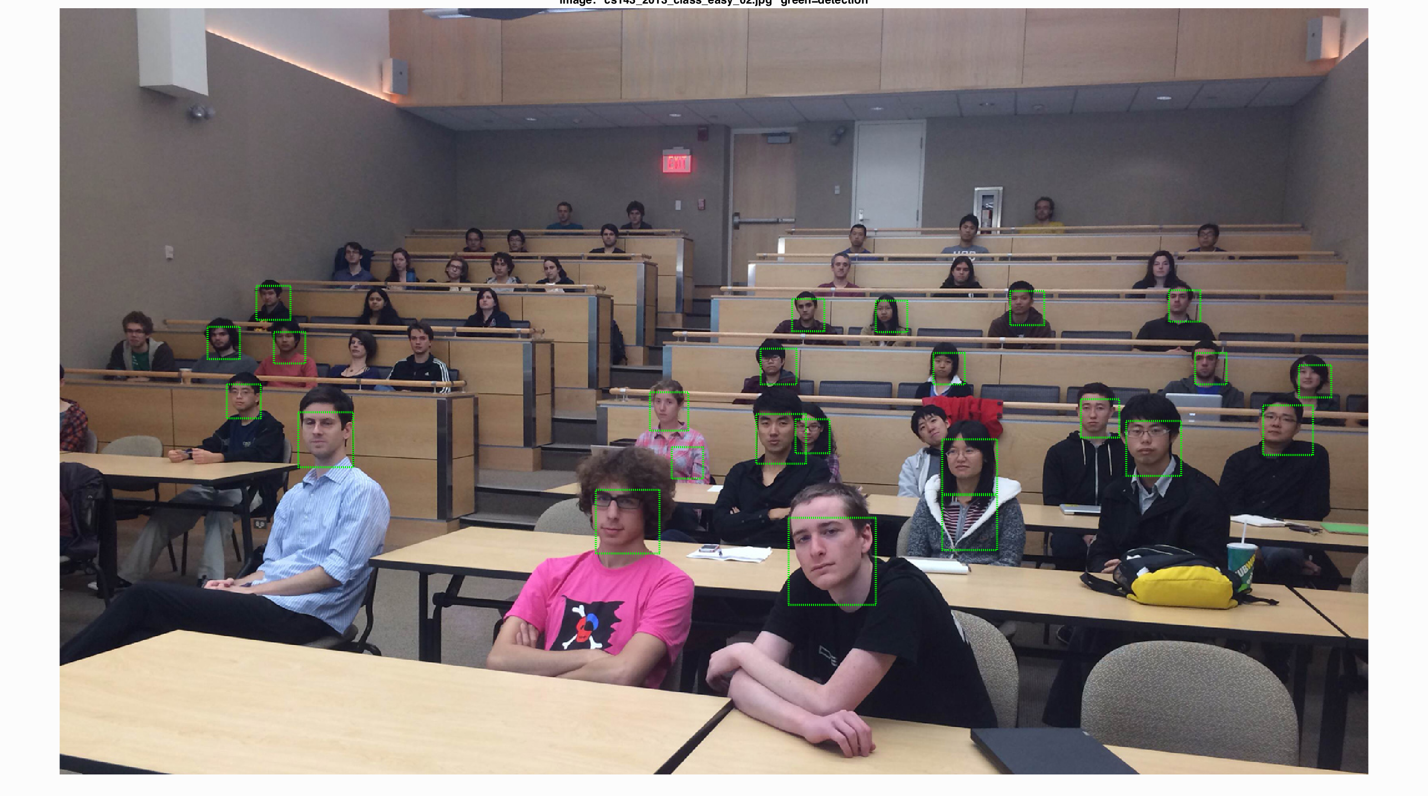
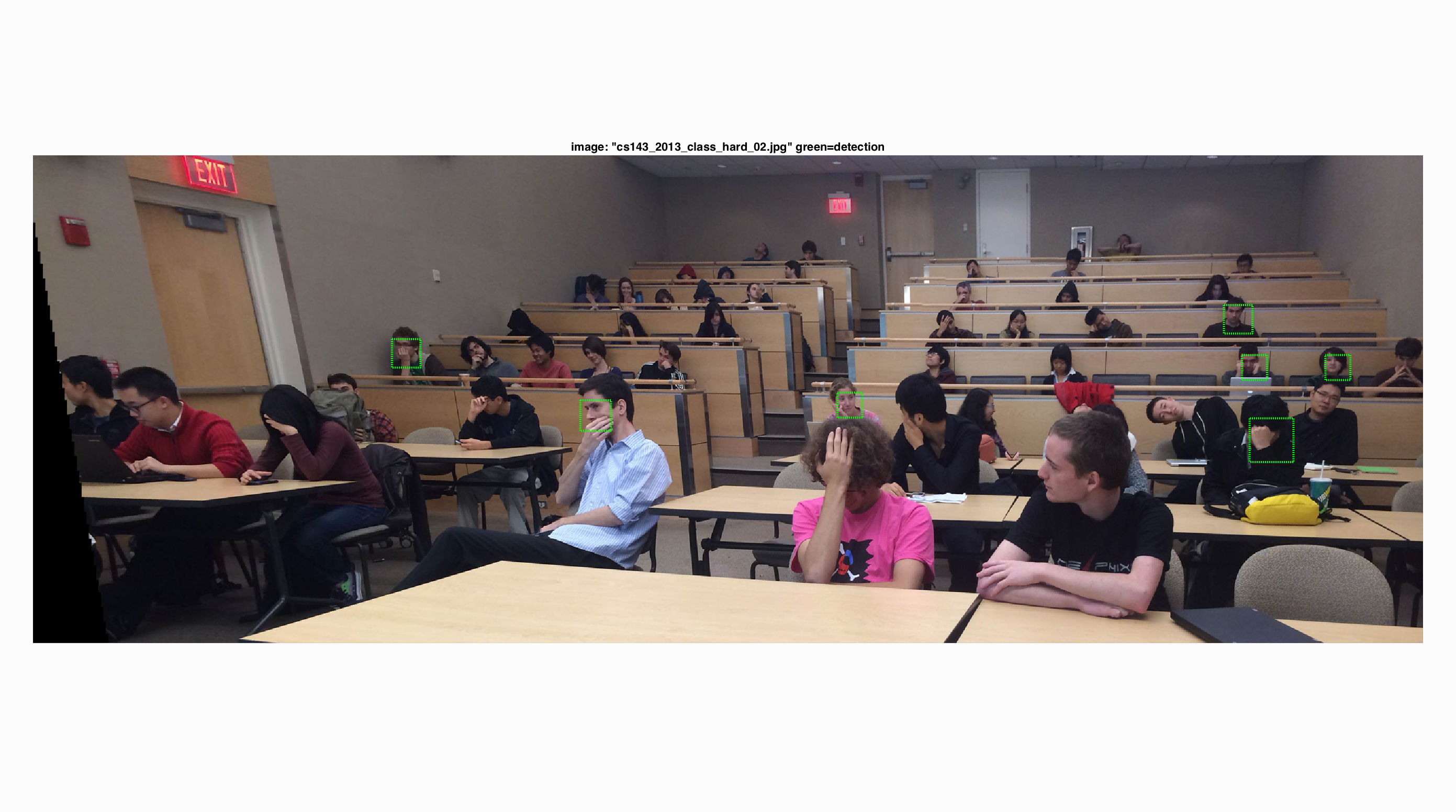
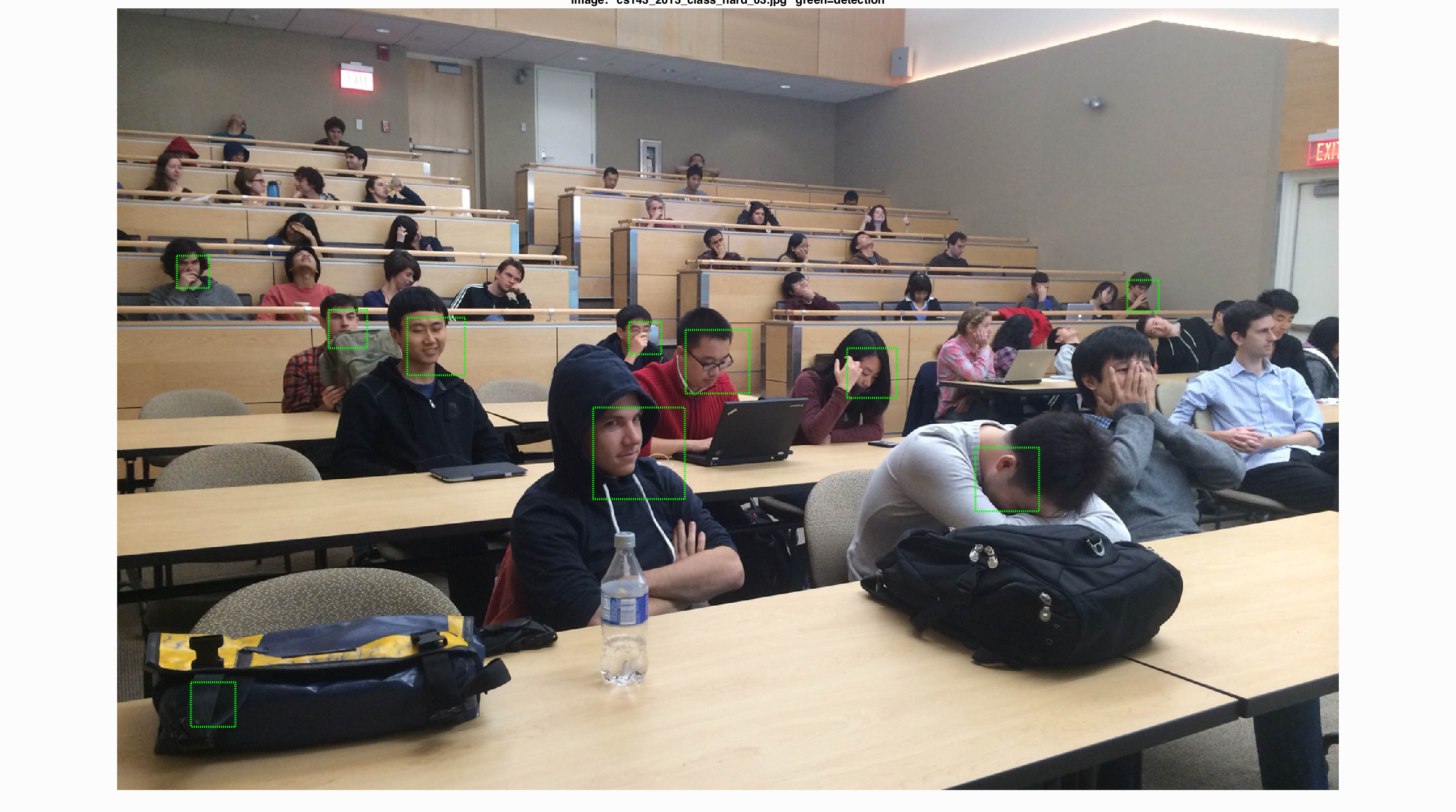
Examples of detection on the test set.